Graphs are a pictorial way of presenting information about quantities which change. Such changes are accurately described in a Table of Figures but even experienced experts can derive information from only relatively small Tables.
Perhaps the most spectacular use of graphical display is the ubiquitous television screen. Here, information is delivered as a sequence of dots (red, blue and green) at a rate around 5-million per second. It is impossible for the human brain to deal with such a stream of information but, when, those dots are properly displayed, we become aware of an image — in fact of 25 images in each and every second.
In the language of graphs there are two (sometimes more) variables or quantities which change and these come in two types:
(a) the independent variable which is always represented by the letter x and which, as its name implies, can assume any value.
(b) a dependent variable which is always represented by the letter y and whose value depends on the value assigned to x.
The value of y is determined by the value of x according to a Rule which is expressed as an algebraic equation. For example the simplest of equations
y = x .........(i)
tells us that, whatever value is assigned to x, that too is the value assumed by y. A slightly more complex form
y = x + 2 ...(ii)
tells us that, whatever the value assigned to x, the value assumed by y is the same va1ue but increased by 2. Similarly the equation
y = x - 3 .... (iii)
tells us that, whatever the value of x, the value of y is that value decreased by 3.
The interesting thing about such equations is the manner in which y changes as the value of the independent-variable is changed and this is not at all apparent until the complete set of values are displayed simultaneously.
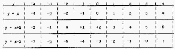
To present the above equations as a graphical display it is first necessary to determine the values of y for each value of x (over the range of interest) and this is laid out in tabular form in Table-1:
TABLE 1
Table-1 shows, along the top line, all the values of x (in this example whole numbers only) ranging from -4 though zero to +4.
The second line shows all the corresponding values for y under the Rule that y = x.
The third line shows all thc corresponding values for y under the Rule that y = x + 2.
The fourth line shows all the corresponding values for y under the Rule that y = x-3.
To plot these figures as a graph Table-1 is turned into a geometric form by representing each figure as a line of appropriate length. Nothing in the Universe is absolute and so a first requirement is to define a point from which all measurements are to be taken. Such a point, marked on a piece of paper, is usually labeled "0” or nought.
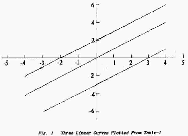
The next task is to construct a frame of reference — a pair of axes (the plural of axis) one of which is to represent the values of x and the other to represent the values of y. Both axes must share the reference point and so they are drawn mutually-perpendicular as shown in Fig. 1.
The horizontal axis is always used to represent the independent—variable and so the vertical axis sn always used for the dependent-variable.
Positive values for x are always plotted to the right arid positive values for y are always plotted upward.
Starting from zero each axis is marked off at equal intervals whose length is determined arbitrarily by the greatest number which it is required to plot along that axis. Clearly the bigger the intervals the more accurately the numbers can be represented.
A pair of figures which represent the corresponding values of x and y (taken from a Table such as Table-1) are known as co-ordinates and, in general, they are written simply as 2,4 meaning that x = 2 and y = 4. When a point is plotted from these figures on perpendicular axes as shown in Fig.1 they are properly called Cartesian Co-ordinates. (There are other ways of plotting graphs.)
As already explained the co-ordinates 2,4 represent the values to be assigned to x and y respectively. To plot such a point move first from "0” to the right along the horizontal x axis to the position marked “2” and then travel upward parallel to the vertical y axis until level with the position marked “4”.
(Alternatively the point is marked at the top of a vertical line 4-units in length which stands at position "2" on the x axis. Yet again you may prefer to think in terms of vertical lines parallel to the y axis and horizontal lines parallel to the x axis.)
The process is repeated for each value of x and, from Table-1, for each of the three equations. Each set of points is then joined by a continuous line to produce the three "curves" illustrated in Fig. 1.
The first thing to notice about these curves is that, in fact, they are straight lines and, as a result, the basic equations are referred to as linear equations. Linear equations deal only in terms which are raised to the power of one [see Lesson-2 in this Part]. Equations which include terms such as x2 produce plots which are curved and which show a single maximum or a minimum value. Equations with terms raised to the power 3 (cubes) produce curves with two reversals - one maximum and one minimum va1ue. In general the number of reversals is one less than the highest power present in the equation.
The second point to note is that all three curves slope upward and to the right; this is because the equations all relate to values of y which increase as x increases. Such curves are said to have positive slopes or positive gradients. This is dealt with again under 7.3.5 Negative Slopes.
The third point is the intercepts which are the values at which the curves cut either or both axes. The simplest equation x = y passes through the origin (the common point which represents zero on both axes) and so both intercepts are zero. This can be deduced by making the independent- variable equal to zero; the corresponding value for y is zero and so the curve must intersect both axes at the origin.
When x is made zero in the second equation the value of y becomes 2 and so the curve intersects the vertical axis (where x = 0) at the point y = 2. Similarly, in the third equation, when x is made zero y becomes -3 and so this curve intersects the vertical axis at the value "3 ” below the origin.
Have you realised that these linear curves have other intercepts because, unless the curve passes through the origin, it must cut both axes. To find these points put y equal to zero. Thus, in. the equation y = x + 2, for y to be zero x must have the value -2. In the third equation, for y to be zero, x must have the value +3.
This demonstrates a useful property of linear curves :
(i) they are straight lines and so
(ii) they can be drawn by calculating the intercepts and joining them with
a ruler.
Inspection of the curves and Table-1 shows that the last two are but the first one either raised by 2 or depressed by 3. A plot of y = 2 is simply a straight horizontal line drawn through the point “2” on the y-axis which is another way of saying that, in this equation, y is not affected by the value of x. Thus the plot of equation (ii) is the result of adding 2 to each value of y; i.e. of summing the two curves ( y = x ) and (y = 2) to produce the equality y = x + 2.
A curve with a negative slope can be obtained by modifying equation (ii) above in that x is given a negative value:
y = -x + 2 ............ (iv)
which leads to a set of values for y shown in Table-2
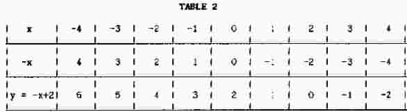
As might be expected reversing the sign of x has caused the va1ue of y to decrease as x increases in value. When this is plotted as in Fig.2 the curve slopes downward and to the right.
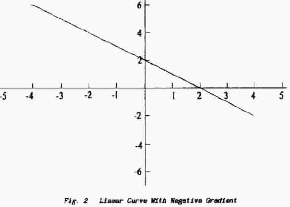
The terms negative slope and positive slope are so named because we regard the slope as the tangent of the angle contained between the curve and the x axis (see Lesson-1: Trigonometry in this Part). Gradients are defined as so many units rise (measured on the y-axis) for so many units of travel (measured on the x axis) - e.g. 1 in 3* - which, in Figs. 1 & 2, becomes y/x.
*In road work the gradient is more usually defined as the number of units rise in so many units along the road; here gradient is the sine of the angle contained between the road surface and the horizontal.
In Fig.2 the independent parameter x is increasing from 0 to the right while the value of y decreases toward 0 (downward). Changes of y in this manner are given negative values and so the ratio y/x becomes negative. In the same manner quantities moving to the left (either decreasing positive values or increasing negative values) are given negative signs; on the y axis negative signs are given to values which “decrease” downward either toward 0 from a positive value or away from 0 with negative va1ues.
I hope it is clear from the above that the equation
-y = x + 2 ............. (v)
must also produce a negative slope ? Note that
-y = -x + 2 ........... (vi)
has a positive slope but it is the same curve as equation y = x - 2. Try plotting it.
(The Rule in algebra is that quantities may be transferred across the equals sign provided the sign is changed. To derive equation (vi) from equation (y = x - 2) take ALL the terms across the equals sign. See Lesson-4: Algebra in this Part.)
A more ambitious equation might be
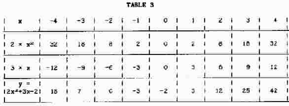
y = 2x2 + 3x - 2 ............(vii)
This equation contains a term in x-squared (raised to the second power), a term in x (raised to the power of 1) and a term (2 x 1) in which x has been raised to the power 0; i.e. it has been reduced to the value 1; see Lesson-2: Powers, indices, etc.A set of solutions is determined in Table-3: note that, when a negative quantity is squared (i.e. it is multiplied by another negative quantity) the result is positive; see Lesson-4: Algebra and also Lesson-7: The j-Notation.
This curve is plotted in Fig. 3. The squared term results in the value of y increasing for both positive and negative values of x and it is this which makes the curve show a minimum value. Those familiar with Calculus will know that the value of both x and y can be calculated for the minimum value because, at the minimum, the gradient of the curve is zero; i.e. the curve is at the point where the gradient changes from negative to positive.
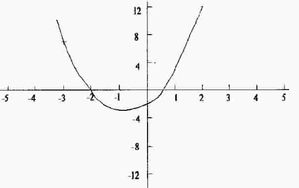
Fig. 3 Plot of an Expression Which Contains a Squared Term
Plot the following equations:
y = x3 + 4x2 + x - 3 y = x5 + x3 - 5x
NOTE: The last curve should show 2 minima and 2 maxima.
In practical work it is seldom required to plot a curve from an equation; if anything it is more likely that an equation is to be derived from a practical curve. Curves are plotted point by point as measurements are taken from a piece cf equipment under test; this is much quicker than tabulating the results first but, because it provides an instant assessment of performance, it enables a test run to be abandoned when it becomes obvious that all is not well. (See also Part-6: Lesson-4: Sweep Oscillator. )
There is always a compromise to be made between accuracy of plotting and the range to be accommodated. For example, when testing an amplifier, interest may lie in the manner in which gain varies as the frequency changes. For a 10.7 MHz IF-amplifier the frequency range may be around 10-MHz to 11.5-MHz and this is easily accommodated on a linear scale such as that above. However, for an AF-amplifier ranging from 30 Hz to 16-kHz there is a problem in paper size. In this instance the scale has to be compressed by calibrating the x-axis logarithmically - this is described below.
Gain - dependent on frequency - will be plotted on the y-axis. However we are not so concerned with the actual output-variation of an audio amplifier as with the manner in which the human ear perceives those variations. The minimum change in sound level which the ear can perceive is 3-dB which is a power-change of 2:1 (see Lesson-2 in Part-7). To achieve a further noticeable increase it is necessary to double the output again. In a manner of speaking therefore we are interested in the ability of an audio amplifier to continuously double its output power.
Output levels can be expressed as 20, 21, 22, 23, 24, ..... and this is a Power series or a Logarithmic series; such a series is used in Lesson-2 of Part-7 to derive the decibel scale. Note that, although the output is rising by leaps and bounds, the indices - the powers of 2 - are increasing in steps of 1. In other words the indices form a linear series; thus the output in decibels can be plotted on a linear scale or the output in volts, amps, or power can be plotted on a logarithmic scale with the same result.
There is one more practical point. Suppose that, for some reason, it was required to plot power-dissipation against current. From Ohm's Law the power is a square-law function of current namely P = I2.R. In performing the experiment there are bound to be experimental errors which cause some of the plotted points to lie off the true curve. As seen in the above examples curves which involve powers soon depart rapidly off the paper. Thus a curve has to be drawn accurately through points scattered around a true curve which is rapidly approaching the vertical.
The easy answer is to plot the results of power measurements on a logarithmic scale and so turn the curve into a straight line: this can then be drawn as best fit using a ruler. Alternatively the equation is re-arranged by taking logs of both sides:
logP = 2. logI. k (k has a constant value)
when logP can be plotted against logI on linear scales with the same result.
A logarithmic scale is marked off in equal distances but the points are calibrated in terms of indices rather than in the figures which they represent. The scale repeats endlessly and the major divisions may be marked (for example) as 1, 10, 100, 1000, 10,000, etc.: the equal spacings represent the logarithms of these numbers. Note that such a scale does not pass through zero; on a logarithmic scale zero is represented by minus-infinity. The scale is selected to cover the range of interest.
Graph paper is printed in linear/linear, log/linear, linear/log and log/log formats.
Back to Top of PageEND OF LESSON