A wavemeter is a device for measuring frequency but it derives its name from the world of physics where, historically, it was easier to measure e-m waves in terms of wavelength.
Suitable frequency-checking equipment is mandatory in an Amateur-radio Station and details can be found on the last pages (Appendix-C) of the DTI document How to Become a Radio Amateur. A general-coverage receiver which incorporates, or which can be used in conjunction with, a crystal calibration-oscillator will suffice but it should be remembered that the frequency-range of measuring equipment must be such as to cover the second and, preferably the third, harmonic of any carrier which the station may radiate.
The following sub-sections describe the different techniques used to measure radio frequencies. Basically the signal under test may be injected into a pre-calibrated variable resonant circuit, heterodyned against a variable calibrated signal-source or the number of cycles executed in one second can be counted.
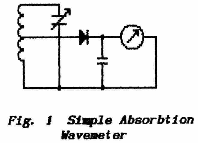
This instrument consists of an L-C resonant circuit which can be tuned over a band of frequencies. The resonant circuit is coupled to some form of indicator to show the presence of current in the circuit. A simple form of absorption wavemeter is shown in Fig. 1. A diode detector, tapped down the inductor to reduce damping, has as its load a capacitor and a dc-meter.
|
The signal under test is coupled usually to the inductor and the tuning capacitor is rotated until, as the circuit resonance approaches the frequency of the signal, power is absorbed from the test signal. The resulting circulating current reaches a maximum value when the circuit resonance is adjusted to the frequency of the signal. |
This condition is indicated by a maximum deflection of the meter. A sensitivity control may be included for convenience, either by shunting the meter with a variable resistor or by including such a resistor in series with the meter, but it is not strictly necessary because the operator can control the degree of coupling to the circuit under test. Alternatively a diode shunted across the meter can be used to create a logarithmic scale.
>>>>>>>>>>>>>>>>>>>> PAGE 2 <<<<<<<<<<<<<<<<<<<<
Go to Top of PageA simple arrangement of this type has a lower limit to its sensitivity because there is a minimum voltage at which the detector diode conducts. This could be overcome by interposing an rf-amplifier between the wavemeter and the diode (but see below) or it is possible with modern op-amps to build detectors which do not suffer these threshold effects.
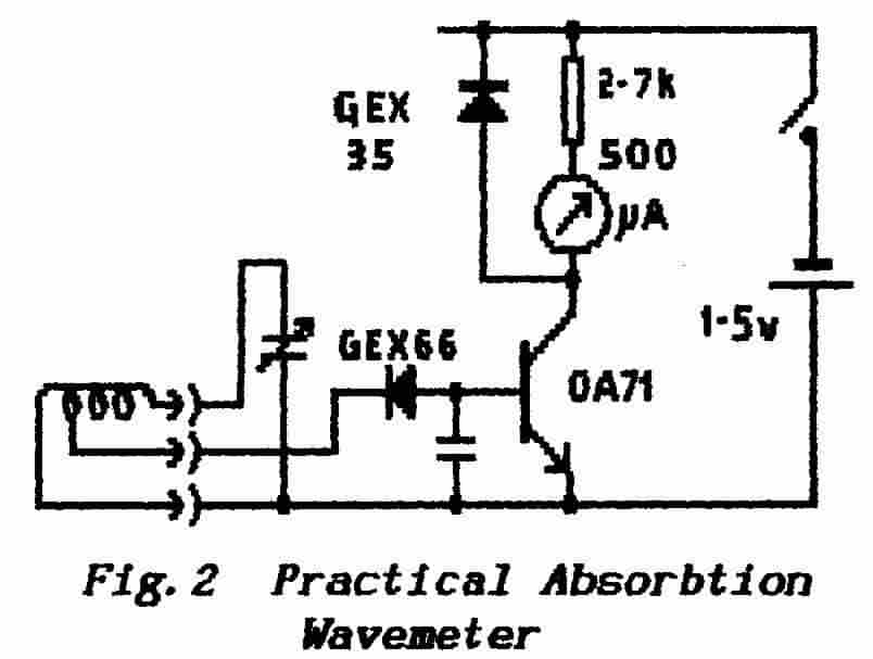 |
In practice sensitive wavemeters can be built by simply interposing a dc- amplifier between the detector and the meter. Fig. 2 shows such an arrangement as built by me some 50-years ago and still giving very good service not only as a wavemeter but also as a probe with which to go hunting for spurious oscillations. A range of inductors are plugged into the hand-held unit to form a probe. (I have no doubt that its performance could today be enhanced still further by replacing the transistor with a FET-input op-amp.) |
** Note that a resonant circuit responds only to that frequency to which it is tuned. The Absorption Wavemeter therefore does not respond in either a harmonic or a sub-harmonic mode and so its primary function is the positive identification of a fundamental frequency.
** The disadvantage of the above simple Absorption Wavemeter is the inability of the diode to conduct below a threshold value (about 0.2-volts for a germanium diode and about 0.6-volts for a silicon diode). It is useless for example for identifying the frequency of a carrier incoming on an aerial (unless the transmitter is very local). The solution suggested above, that a rf-amplifier be interposed between source and wavemeter, is self-defeating because such an amplifier could certainly generate harmonics at a power-level sufficient to register on the meter.
** The accuracy of absorption wavemeters is limited by the ability to read the calibration marks on the dial.
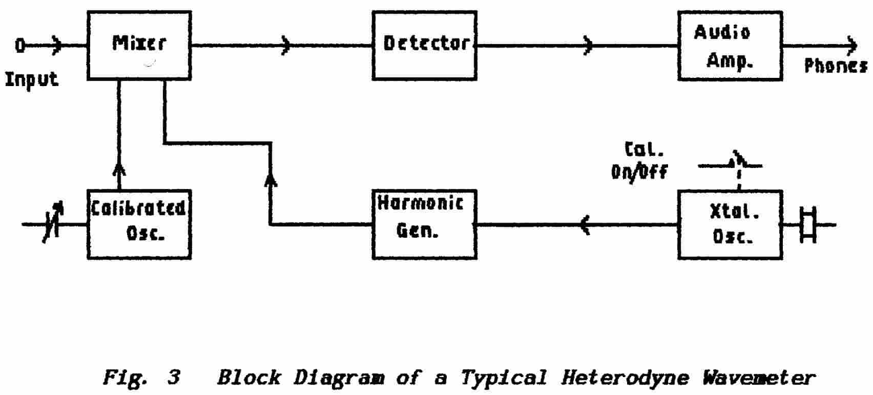
These wavemeters use a calibrated oscillator that feeds into a mixer circuit together with the signal under test. The two signals beat as described under 2.2.5 and 2.7 and the result is passed to a detector-circuit and thence to either headphones or loudspeaker. In principle these wavemeters are but carefully constructed and calibrated superhet receivers.
** The audio output from a frequency-translator and detector combination is proportional to the amplitude of both the input and the (strong) local-oscillator signals. Thus these wavemeters can be very sensitive indeed and easily respond to signals incoming on an aerial. They also offer greater accuracy than the absorption types in that built-in crystal oscillators with harmonic-generators enable the calibration scale to be checked at intervals ; generally a moveable cursor is incorporated so that the scale can be adjusted over the frequency-range of interest.
>>>>>>>>>>>>>>>>>>>> PAGE 3 <<<<<<<<<<<<<<<<<<<<
Back to Top of Page** The disadvantage of the Heterodyne Wavemeter is that it is extremely sensitive also to harmonics of the signal under test and also produces responses to spurious signals that arise from (a) beats between the test-signal and the L.O.-harmonics and (b) beats that arise between harmonics of the signal and of the local oscillator. These often appear to be sub-harmonics.
** It follows therefore that, to measure the frequency of a signal, an absorption wavemeter is required to identify the fundamental (unless it is already known) and then a heterodyne wavemeter can be used to obtain a degree of accuracy. A block diagram of a typical wavemeter is given in Fig.3.
** These instruments use digital-circuit techniques to actually count the number of cycles which occur in a defined period. A typical Counter is shown in block-diagram form in Fig. 4. The essential component of these instruments is a gate circuit which blocks the passage of a signal until the gate is "Opened" by a suitable pulse. The gate remains open until it is closed by a second pulse or perhaps by termination of the pulse that was holding it open.
** The signal to be measured is applied to the gate-input ; if the gate is held open for exactly 1-second then the number of cycles which are passed to its output represents the frequency in cycles-per-second (Hz).
The number of cycles to be counted can be varied by adjusting the gate width (sometimes referred to as the "time-base"). For example a 1-MHz carrier would produce a count of 106 with the gate set to 1-second . A 100-MHz carrier would produce the same count of 106 with the gate set to 10-milliseconds (10 ms). Thus the control which sets the gate-width becomes a multiplier to be used in conjunction with the display. The 10-ms position would be labeled " x 100 " .
>>>>>>>>>>>>>>>>>>>> PAGE 4 <<<<<<<<<<<<<<<<<<<<
Back to Top of Page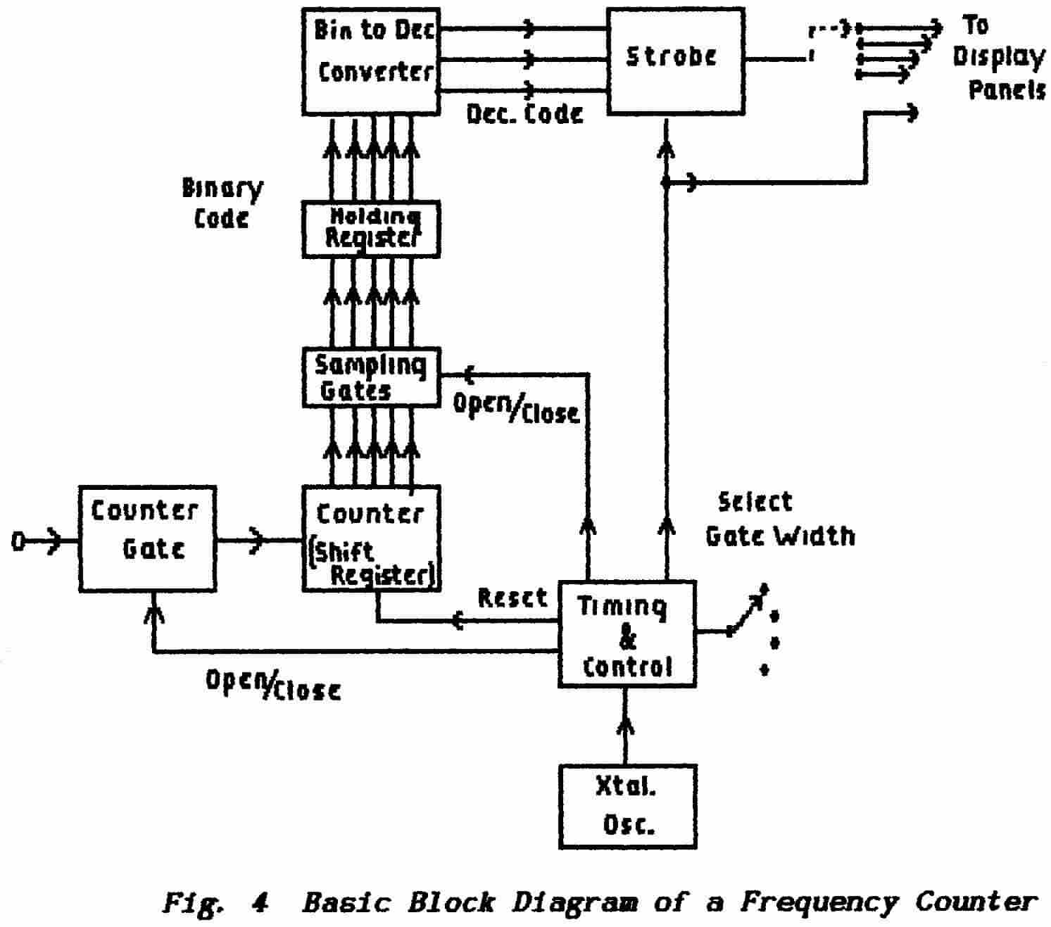
The output from the gate circuit is applied to a shift register as described in Part-2, Lesson-4 under 2.2.9 The Binary Counter. When the gate is closed the condition of the various stages of the Counter indicate, in binary form, the number of cycles which passed through the gate. The count is held for a short period, the Counter is then reset to zero and the gate re-opened so that the frequency is continually monitored for any change.
During the period that the count is held in the Register the result is sampled by opening another gate - in fact a set of gates one for each stage of the Counter; the count is transferred (a parallel transfer) to a second "holding" register for processing while the counter is recycled. The connections from this second register are arranged so that the binary number is converted to a decimal number before being passed to the display.
The display consists basically of a number of panels each of which contains a number of light-emitting diodes (L.E.D.s) arranged in a pattern such that, by energising an appropriate combination of diodes, any required number can be simulated. There is one of these panels of diodes for each digit to be displayed. ( Alpha-numeric, or "starburst", panels are available which can display letters of the alphabet as well as numerals.]
The complex process of selecting the requisite L.E.D.s is undertaken by specially designed chips. The display is constantly "strobed" at high-frequency so that each panel of the display is illuminated in sequence: to increase the display brightness the strobe frequency is increased. At each pass the panels are corrected (up-dated) according to the latest count from the counting register.
>>>>>>>>>>>>>>>>>>>> PAGE 5 <<<<<<<<<<<<<<<<<<<<
Back to Top of PageSpecial transmitters have been set up whose purpose is to radiate a signal the carrier-frequency of which is controlled to a very high degree. Their intended purpose is frequency-measurement by heterodyne methods.
The grid-dip oscillator (or grid-dipper) is a simple tool with two basic functions which, in today's all-semiconductor world, is seemingly misnamed. It is an absorption wavemeter but, by switching-in an active device, it can be used also "in reverse" to determine the resonance frequency of an LC circuit.
** A typical circuit in its original form is shown in Fig. 5. To
achieve a wide frequency-coverage the instrument is provided with a range of
plug-in coils ; thus, to simplify the coil construction, the circuit
is shown as an inverted Colpitts oscillator. A milliammeter is connected in
series with the grid leak where it measures the grid current.
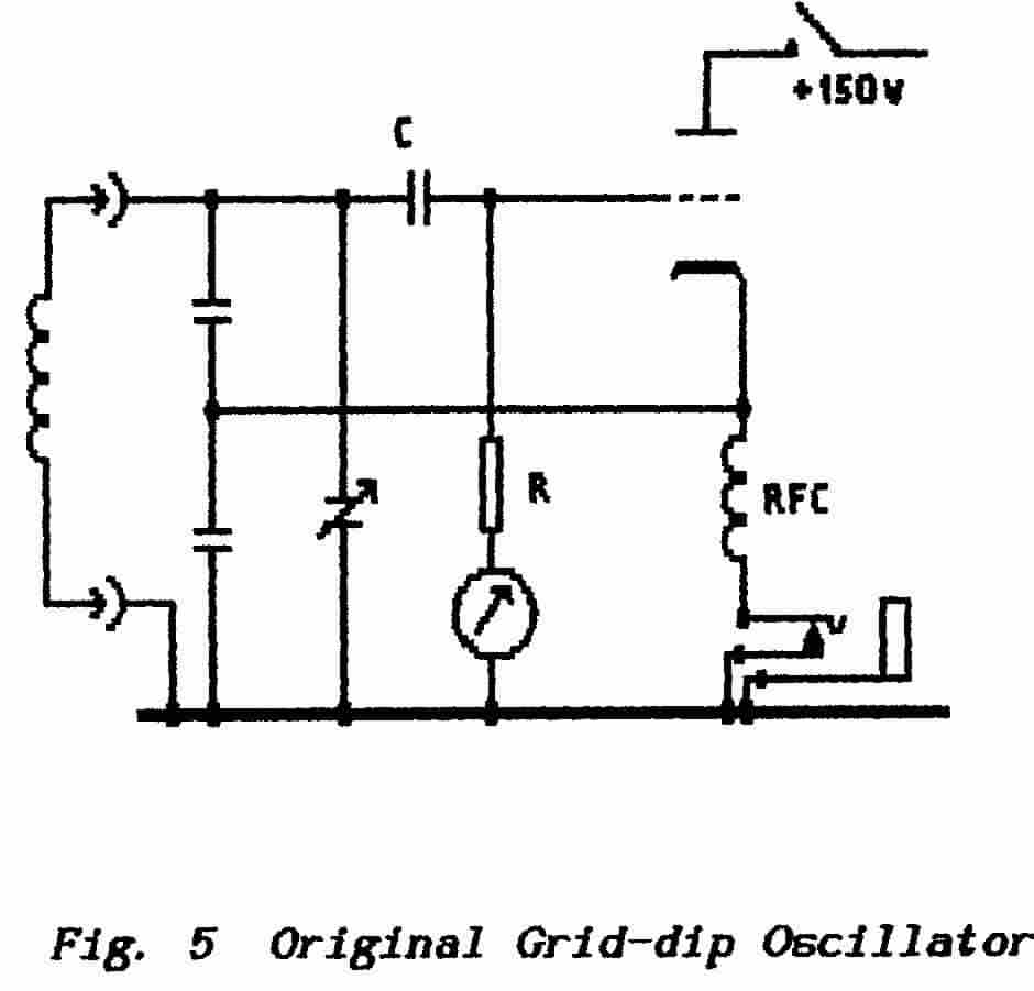 |
** As an oscillator its action is controlled by the RC bias-combination in the grid circuit. With the coil close to the circuit under test the capacitor is varied to adjust the frequency of oscillation ; as this passes through the resonance frequency of the test circuit so that circuit absorbs power from the oscillator. This power-loss lowers the amplitude of the oscillation and this decreases the bias which appears on the meter as a drop in grid current. This is the "grid dip". The Meissner circuit is often used in G.D.O. construction. |
** When the switch in the anode circuit is opened the oscillation ceases. The instrument can then be used as an absorption wavemeter with the grid-cathode acting as a diode detector and the meter as the indicator. With a pair of headphones or a loudspeaker plugged into the anode-circuit jack and the switch closed the device also serves as an inaccurate heterodyne wavemeter. With the switch open it serves as a signal monitor/tracer.
** A disadvantage of this device is the requirement for a power supplier but this is less serious when the active device is a transistor or op-amp and an internal battery can be utilised. However, it is a good idea to fit a L.E.D. indicator to warn that the battery-switch is closed.
>>>>>>>>>>>>>>>>>>>> PAGE 6 <<<<<<<<<<<<<<<<<<<<
Back to Top of PageThe G.D.O. comes into its own on the constructor's bench where it can be used to determine the number of turns required in setting-up LC circuits and also in chasing spurious oscillations. It is particularly useful in that it can provide measurements on circuits yet to be completed and which therefore cannot be powered.
END OF LESSON 1
* * * * * * * * * * * *
QUESTIONS
1. Outline the D.T.I. amateur radio station requirements for measuring facilities in an amateur-radio station.
2. Give the advantages and disadvantages of an absorption wavemeter.
In place of an indicating meter an absorption wavemeter is fitted with a small lamp. What is the likely intended use for such an instrument?
3. What is the major purpose of a heterodyne wavemeter?
4. Give the basic functional details of a frequency—counter instrument. (You are not required to describe the internal workings .)
5. A Counter is displaying 157.00582 kHz with the Multiplier set to x10, What is the frequency being measured ?
6. You are presented with a brand-new superhet receiver which has a poor response. How would you use a G.D.O. to check a suspicion that the aerial-input circuit was in fact operating on the wrong ranges?
>>>>>>>>>>>>>>>>>>>>>>>>>>>> PAGE 7 <<<<<<<<<<<<<<<<<<<<
Back to Top of PageAn analogue meter is one which measures a quantity by analogy ; most analogue meters represent the magnitude of a parameter as an angle of rotation but some show it as a linear (straight line) motion.
The most common of meters is the moving coil meter in which the electric current to be measured is passed through a lightweight coil. The coil is suspended on pivots in the magnetic field of a permanent magnet. As shown in Fundamentals-1 Lesson-4 coiling a conductor collects the magnetic field into the same form as that of a bar magnet. The two magnetic fields interact and a torque (a rotational force) turns the moving coil so that the fields are aligned. A pointer attached to the moving coil indicates the degree of rotation.
As described so far the meter is useless because any current of whatever value would cause the two magnetic fields to align end so produce the maximum possible deflection. The coil is restrained by a small spring and the rotation is checked when the tension in the spring exactly balances the torque set up by the test current. An increase or decrease in the current causes an increase or decrease in the torque and so the coil deflects through a greater or lesser angle until there is sufficient tension in the spring to balance the system once more.
[Note that the function of the spring is not to return the pointer to zero when the current is removed ; it is an essential part of the meter- action.]
The resistance of the coil is very low and so care must be taken to limit the applied voltage. The magnitude of the full-scale-deflection (f.s.d.) current can be controlled by selecting the tension of the spring but this is limited by the load imposed on the pivots.
The f.s.d. current is increased by connecting a meter shunt in parallel with the meter so that excess current flows around the meter rather than through it. The value of the shunt resistance (Rs) is related to the coil resistance (Rm) in the same (but inverse) ratio as the current through the meter (Im) is related to the current (Is) which flows through the shunt
Rs/Rm = Im/Is
where of course the shunt-current equals the total current less the meter current.
These meters are adapted for use as voltmeters by connecting a multiplier resistor in series. This resistor is chosen so that the voltage dropped across the multiplier equals the full applied voltage less that dropped across the meter coil. In general the voltage across the meter is so small compared with that across the multiplier that the meter resistance can be ignored ; however, for accurate measurements (a Grade-I Meter) the meter resistance must be taken into account.
>>>>>>>>>>>>>>>>>>>> PAGE 8 <<<<<<<<<<<<<<<<<<<<
Back to Top of PageThese meters are adapted also for use as ohmmeters by including a small battery in circuit. The meter indicates the current which is driven through the resistor to be measured ; because the terminal voltage of the battery is known the meter scale can be calibrated in ohms instead of amps.
There is a problem here in that the terminal voltage of a practical battery is not constant throughout its life. This is overcome by including a small variable resistor whose function is to reduce the voltage from the battery. Before making a measurement the meter connecting-leads are first connected together (zero ohms) and the variable adjusted for f.s.d. — this point is Zero on the ohms-scale.
These three basic functions (and others too) are incorporated into a single instrument known as a multimeter in which the different modes (amps, volts, ohms) are selected by switches and also a number of ranges are offered by switching different shunts and multipliers.
The basic instrument can measure only direct quantities but it can be adapted for ac measurements by including a small rectifier unit (usually a bridge rectifier — see Part-5). There are three things to remember when using such an instrument on ac:
(a) the instrument can be calibrated to indicate either the peak waveform voltage, the average voltage or the rms voltage (see Part-7)
(b) the instrument will function satisfactorily only up to a frequency which depends on the effects of stray capacitance and stray inductance within the instrument
(c) the reading given by the instrument will be affected by the waveform of the signal ; i.e. distortion will change the rms, average and peak values. Normally meters are calibrated in terms of rms values for a sinewave.
Rough measurements of capacitance can be made by measuring the ac-current which a capacitor passes for a known applied voltage. Power is measured (within the frequency range of the Instrument) by dissipating the applied energy in a known resistive load and using the meter to indicate the voltage developed across that resistor.
Switches are both expensive and troublesome and sometimes the mode switch is dispensed with — or simplified — by providing alternative connections to a multimeter.
Multimeters require care in use because it is too easy to attempt a voltage measurement with the instrument set for current measurement. The disadvantage of the versatile moving-coil (rn-c) meter is its lack of robustness.
Delicate rn-c meters (say up to 1-mA f.s.d.) should always be kept with their terminals connected together when not in use ; good quality electronic rnultimeters (see next section) arrange for such a short-circuit connection to be made when the instrument is switched off. The short circuit allows current to flow when the meter-movement is disturbed ; the coil, moving within the permanent magnetic field, acts as a generator. The magnetic field which results reacts with the permanent field and forms a braking action on the movement which protects it from damage.
>>>>>>>>>>>>>>>>>>>> PAGE 9 <<<<<<<<<<<<<<<<<<<<
Back to Top of Page A serious disadvantage of the moving-coil meter
is that it demands a current from the circuit under test. Connection of such
a meter therefore changes the conditions in the test circuit and so produces
a false reading. This is demonstrated in Fig. 6.
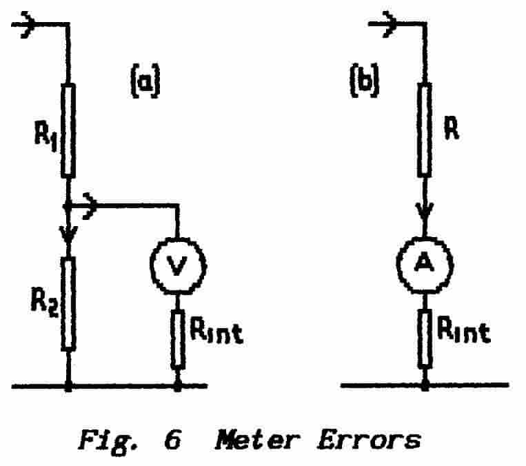 |
** Diagram (a) shows a simple potential-divider network
with a voltmeter connected across the lower half. There are two ways of
considering this circuit: (a) the current drawn by the meter is added to that drawn through the upper resistor and so it lowers the voltage at the junction. (b) the meter resistance is in parallel with the lower resistor and so the lower resistor is effectively reduced in value : because the potential divider has been modified the potential at the junction is lowered. |
** Diagram (b) shows the error caused by attempting to measure the current. The resistance of the meter is added to that of the resistor and so the circuit current is reduced. If the resistor has a value at least 10-times that of the meter the error is not likely to be significant in practice but, where errors below 10% are cause for concern, it is necessary to calculate the correct result from the meter reading.
Clearly the addition of multipliers changes the overall resistance of a meter and, in a multi-range multimeter, some criterion is required to describe the overall resistance. The value of each multiplier depends on the f.s.d. current of the movement and on the intended f.s.d. voltage for a particular range. For example, if the instrument uses a rn-c meter with a f.s.d. of 100 μA then, by Ohms Law, on the 10-volt range it will present a resistance of 10/0,0001 ohms or 100 kilohms.
On the 100-volt range its resistance will be 100/0.0001 or 1 megohm. This linear relation between f.s.d-voltage and overall resistance is expressed as 10-kilohrns per volt. Had the multimeter been constructed using a rn-c meter of 1-mA f.s.d. then the multimeter would have been quoted as 1-kilohm per volt.
In complex circuits the effect of connecting a low-resistance meter can have far-reaching results and this is particularly so in circuits which employ dc-feedback loops which are very common in modern electronics.
>>>>>>>>>>>>>>>>>>>> PAGE 10 <<<<<<<<<<<<<<<<<<<<
Back to Top of PageThis description today usually means a digital meter (described later) but the operation of those is much more sophisticated.
The electronic multimeter drives the analogue
device through a dc-amplifier and it is not too difficult to arrange that the
amplifier presents a very-high impedance at the input terminals. Range-changing
can be effected both by use of multiplier resistors and by changing the amplifier
gain usually by switching the feedback circuit. For current measurement a set
of shunts must be provided across the meter input but this is a straightforward
matter because the instrument does not draw current from the test path. The
difficulty with these instruments however lies in designing the dc-amplifier
so that it does not suffer from drift problems with changes in ambient temperature
or changes in the power-supply. In addition high-impedance circuits are very
prone to pick-up hum.
Analogue meters in all forms offer the great advantage of giving a pictorial display of circuit conditions. It is immediately obvious that the current is either rising, falling or reaching a steady-state. The greatest disadvantage lies in the inability to read them very accurately.
Consider for example a meter which is calibrated from 0 to 10 mA. It will have 10 major divisions which indicate steps of 1 mA and each of these will most probably be sub-divided into five smaller divisions of 200 μA each. (A physically-large instrument may well be sub-divided into 10 divisions of 100 μA each.) . The eye can distinguish between a half-division and a whole division and so the meter can be read to an accuracy of 100 μA. But that is only part of the story.
When the meter is operated at f.s.d. the error is 100 μA in 10 mA ... or 1%. When the meter is indicating 1 mA the error becomes 100 μA in 1 mA which is 10%. Thus it is important to choose an analogue meter such that it operates at or close to its f.s.d.
These give their indication in the form of an extending line and are most commonly found in LED displays known as bargraphs. Variations of the parameter to be measured are converted to a set of numbers (using an analogue-to digital-convertor or ADC) and each number is represented by an LED in the display. As the parameter rises through each pre-determined level so the appropriate LED becomes illuminated. The display is seldom used for quantitative measurement but only to present a general picture such as signal-level monitoring in a tape-recorder.
The display may take two alternative forms either a bargraph, in which the LED's are illuminated to form an extending line, or a moving-dot display in which only one LED (representing the largest number) is illuminated at any one time.
>>>>>>>>>>>>>>>>>>>> PAGE 11 <<<<<<<<<<<<<<<<<<<<
Back to Top of PageEssentially a digital meter is one which displays its measured result as a number; i.e. a string of digits with a decimal point. However, in its internal workings, it is if anything more analogue than a m-c meter. The nomenclature of these instruments causes puzzlement when reference is made to (say) a 3½-digit display ; the ½-digit is the decimal point.
The first stage in a digital meter is an analogue-to-digital converter whose function is to translate the variable input (analogue) signal into a number. It is this process which gives rise to the meter's drawback. The sampling and ADC process has to be constantly repeated to derive a new number whenever the input value changes.
As explained in the previous Lesson a digital display is illuminated one digit at a time when it is up-dated from the display memory appropriate to the digit. The ADC must keep the display memory in step with the input-signal variations.
When the input signal changes rapidly it may require several cycles of this up-dating process before the meter catches-up with the input signal and so digital displays tend to be confusing in that there is always uncertainty as to whether the result is increasing or decreasing. Some meters incorporate a bargraph display also which gives this information. Often the need to wait until the display settles makes the meter less useful than an m-c instrument. In tuning operations, where the operator is looking for a maximum or a minimum meter reading, a digital meter is fairly useless.
There are several techniques available for digital measurements but a basic idea is given in the following paragraphs for those interested; this is not required for the R.A.E.
A ramp voltage or ramp-waveform is one which steadily increases its value up to a fixed level ; it then rapidly reverts to zero ready to start again. It may be generated by passing a current of strictly-controlled value into a good-quality capacitor. In such a waveform there is a fixed relation between the elapsed time since the waveform commenced and the value to which the voltage has risen. (Further information will be given under Pulse Techniques.)
It is easy to measure time accurately by counting the number of cycles of a crystal-controlled oscillator (see Frequency Counters in previous Lesson). The oscillator waveform is passed through a gate-circuit which is opened as the ramp commences ; counting then continues until the gate is closed after which the display indicates the time (in cycles) for which the gate remained open.
The ramp waveform is applied to a voltage-comparator circuit where it is compared to the voltage of the applied test-signal. When the two voltages are equal the gate is closed. Thus the display (a number of cycles representing elapsed time) also represents the time taken by the ramp to reach the voltage of the test signal. The relation between elapsed time and ramp-voltage is known (in fact it is designed) and so the display can be calibrated in terms of volts.
>>>>>>>>>>>>>>>>>>>> PAGE 12 <<<<<<<<<<<<<<<<<<<<
Back to Top of PageA digital meter can give an accurate reading to several decimal places which is little affected by considerations of f.s.d. as outlined above for the analogue meter. However, its habit of constantly re-evaluating the signal by counting-up from zero makes the read-out somewhat baffling with rapidly-changing signals.
Digital systems are used in the construction of multimeters. They have two great advantages ; (a) their very-high input impedance prevents loading of the circuit under test (b) they can be constructed to limit the voltage they may apply to the circuit under test thus avoiding damage to integrated circuits of the CMOS type.
Electronic meters offer input impedances up to many hundreds of megohms and are a blessing indeed in low-current easily-damaged electronic circuits. At the other end of the scale however, in high-current circuits, they can lead the unwary astray.
Consider a motor-car which refuses to start. On turning the ignition key all the electrics come on but, as soon as the starter switch is engaged, everything dies. Flat battery ? Yes, except that, when the starter switch is released, all the electrics come back to life.
End-of-battery-life is a reasonable diagnosis except that the car behaved perfectly yesterday. Clearly there is a bad connection somewhere which can be sorted quickly with the aid of a meter. Of course, the most convenient meter to use is that handy little electronic digital meter.
Car electrics handle anything up to 35 amps and, in the starter-motor circuit, anything up to 100 amps ; at 35 amps a corroding connection offering only 0.3 ohms would reduce the available battery voltage to 2 volts. After 10 minutes work with the digital meter it is clear that here is another of those electrical nightmares in which there is nothing wrong with the device except that it will not work.
The cure is to put the electronic meter away and do the circuit checking with a spare headlamp bulb and a couple of lengths of wire. Given a dry-terminal resistance of 50 ohms the electronic meter will indicate a good connection because it draws probably 1μA or less — the drop in terminal voltage at 50 ohms amounts to 50 μV. The headlamp bulb requires around 4 amps and it will not function with 50-ohms in series.
In high-current circuits always use a high-current indicator but, above all, keep all connections clean and lightly smeared with vaseline (chassis grease is a good second choice). Finally remember that, in mobile amateur equipment, a current in excess of 20 amps will be drawn by a rig which is transmitting on full power.
>>>>>>>>>>>>>>>>>>>> PAGE 13 <<<<<<<<<<<<<<<<<<<<
Back to Top of PageOne method of measuring power has been indicated already under 6.2.1 wherein the power is dissipated in a resistor of known value and the voltage which is developed across that resistor is measured. Reference to Ohms Law however reminds us that power is proportional to the square of the voltage and so this simple method of measuring power produces a non-linear meter scale which is cramped toward the high-power end.
Nonetheless this system is often used ; I own a RF Power Meter which is simply a resistive dummy-load to which is attached a diode detector and m-c meter. A switchable meter shunt reduces the meter sensitivity to give two ranges 0-50 watts and 0-100 watts.
RF-power has a nasty habit of leaking and, if the power does not reach the dummy load, then it cannot be included in the final power reading. The entire apparatus must be enclosed in a metal screening-box fitted with a coaxial connector so that a coax feeder can be used to connect it directly to the transmitter output. The case must be ventilated and be large enough to transfer the heat to the atmosphere at a rate sufficient to limit the temperature rise.
Additionally the resistive load and its case must be designed so that, over the desired frequency range, it looks like 50-ohms to the feeder else it will set up a standing-wave that will destroy both the transmitter and all possibility of accurate measurement.
The diode detector poses a new problem in that, depending on the frequency, it may act as a peak detector or as a something-less-than-peak detector ; to measure power it is necessary to use rms values (see Part-7). One simple way to calibrate the instrument is to drive it with a direct current because this can be measured, either in voltage or current, with normal workshop meters. For each power setting of the wattmeter the true power can be calculated. This only works of course within the passband set by the stray reactances and the time-constant of the diode detector.
A second method is to sample the voltage or current. A toroidal transformer (see Fundamentals-1 Lesson-5) can be used to extract a small proportion of the rf-current. Alternatively a simple voltage-divider, either resistive or capacitive, can be used to sample the rf-voltage. Provided the resistance of the load is known accurately the power can be calculated. This method has the advantage that detection is carried out at low level.
A more usual method is to use either a directional coupler or a so-called bridge arrangement which forms part of an swr meter. These are described in the next Lesson.
END OF LESSON 2
* * * * * * * * * * * *
QUESTIONS
1. A milliammeter with f.s.d. 1-mA and resistance 120-ohms is to be used to make a simple multimeter with voltage ranges up to 10 volts and 100 volts and current ranges up to 100 mA and 1 amp. Calculate the values of the multiplier and shunt resistors that will be required.
2. The diagram shows a valve with an anode-load resistor of 10,000 ohms. The anode voltage is measured with a multimeter offering 1,000 ohms/volt. On the 200 volt range the meter shows the anode voltage as 140 volts. Is the correct answer 200 volts, 144 volts or 100 volts ?
3. A cell of 2 volts is connected across a 2000-ohm resistor. If the above 120-ohm milliammeter is connected in series what would you expect it to read ? What voltage would a high-impedance voltmeter record across the resistor with the milliammeter in circuit?
4. What is an electronic meter as distinct from a digital meter ?
5. Why would an LED array make a suitable tuning indicator for an A.M. receiver but not be of use in an f.m receiver or as a means of checking the performance of a transmitter ?
>>>>>>>>>>>>>>>>>>>> PAGE 14 <<<<<<<<<<<<<<<<<<<<
Back to Top of PageThe method given under 6.5.1 in the previous Lesson results in a power calculation made from the expression
power = E2/R
The method described here also relies on a calculation but uses the formula
power = I2R
RF current can be measured directly by means of either a hot-wire ammeter or a thermocouple meter both of which rely on the heating effect of an electric current.. There is a frequency limitation however because, as frequency rises, so stray capacitances tend to bypass the heat element.
The Hot-wire Meter A short length of wire is stretched between two anchor points and tensioned at its centre by a cord which, after passing around a pulley, is attached to a spring. The pulley carries the meter's pointer. Any current which flows through the wire causes it to heat and so expand. This expansion is taken-up by the spring which, in drawing the cord over the pulley, moves the pointer. This is a fairly robust meter.The Thermocouple Meter A thermocouple, in simple terms, consists of two dissimilar wires with their junction attached to (but insulated from) a small heater. The current to be measured is fed through the heater which thus heats the junction. Because the junction contains two dissimilar metals an emf is generated whose magnitude depends on the temperature of that junction. The output from this thermo-electric transducer is fed to a sensitive microammeter.
Because these meters depend on the heating effect of a current they register power whether the current is dc or ac. As a consequence they can be calibrated by passing a direct current whose value is easily measured by means of a standard dc meter. They give a true indication of power irrespective of waveform ; (see under RMS Values for a Sinewave in Part-7).
To measure power a dummy load is used as before but the rf-ammeter is connected in series. The power is calculated as I2.R where R is the value of the dummy load. The square law results in a non-linear scale but this is often corrected in the mechanical and/or electrical design.
>>>>>>>>>>>>>>>>>>>> PAGE 15 <<<<<<<<<<<<<<<<<<<<
Fig. 7 shows one form of directional coupler.
It consists of two pieces of coax feeder joined side by side which are coupled
together in two places by allowing the electric and magnetic fields to leak
through holes. All four ends are terminated in coax couplers.
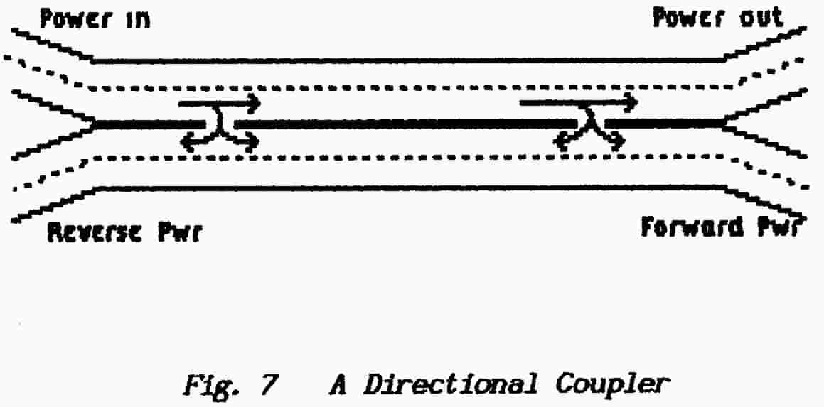
The diagram shows power injected into the left-hand
end of the top cable and removed from the right-hand end. In fact the coupler
can be used either way round with the main power-flow in either cable.
Power which leaks through the two holes propagates in both directions along the second cable. Consider first the power which travels from left to right along the second cable. That which leaks through the first hole and travels to the second hole is in phase with that which leaks through the second hole. Thus the two signals travel together to the right-hand end of the lower cable and add together in whatever load is connected there.
Power which leaks through the second hole but travels toward the left-hand end of the lower cable arrives back at the first hole but is delayed in phase by twice the time taken for the signal to travel the distance from one hole to the other (i.e. there and back). At the left-hand end of the lower cable these two signals tend to cancel ; the degree of cancellation depends on the relation between frequency (i.e. wavelength) and the distance which separates the holes. The device therefore is frequency conscious ; also, if there is to be any appreciable cancellation, the hole-spacing must be comparable in size to the wavelength and this limits use of the directional-coupler roughly to frequencies above 30 MHz.
It is found that, for any given frequency or small range of frequencies, the outputs from the lower cable are a fixed percentage of the power which flows on the main cable. Should the main feeder path be mismatched then the current and voltage relation becomes reactive and this affects the addition and subtraction of signals in the second cable.
The power which emerges at the right-hand end of the lower cable is always a fixed percentage of the power traveling from left to right on the main feeder — mismatched or matched. The power which emerges at the left-hand end of the lower cable is always a fixed percentage of the power traveling from right to left ; i.e. power which is reflected from a mismatched load. Hence a simple subtraction gives the power being absorbed by the load and a comparison of the two outputs enables a calculation of the s.w.r.
>>>>>>>>>>>>>>>>>>>> PAGE 16 <<<<<<<<<<<<<<<<<<<<
Back to Top of PageA directional-coupler has to be calibrated before it is of much use. To do this power is injected at (say) the left-hand end of the cable which is to be the main-feed line ; the other three connections are terminated in matching dummy loads. A sensitive detector (such as a receiver with a calibrated attenuator) is now used to measure the signal levels at the two right-hand end connectors ; this gives the ratio of signal-level on the main line to signal-level coupled-out of the "forward" side-connector. A similar measurement at the "reverse" side-connector should show a very large attenuation of the signal.
The power is now fed along the main feeder in the opposite direction and the process repeated. The directional-coupler is now ready to indicate the forward and reverse power-flows on the main feeder as a proportion of that main flow (this is the Coupler's attenuation factor).
By itself the directional-coupler can now be used for measuring s.w.r. Additionally, when the output level at a side-connector is measured (by use of a receiver and a signal-generator) this can be used with the attenuation-factor to calculate the power-flow on the main feeder. Note that the attenuation- factor must be measured for every (small) range of frequencies
Some directional couplers are made by threading a small length of wire down a section of feeder between the outer and inner conductors. This forms a loop, short with respect to the wavelength, which is inductively-coupled to the main feeder. The voltage/current ratios which are induced along the loop differ along its length and its operation can be argued in a manner similar to that above.
Yet another method is to use printed-wiring techniques to lay down a small length of transmission line which, in appearance, is a balanced feeder. It is used as two separate feeders coupled in the manner of the loop described above.
Note that all forms of directional-coupler are frequency (more accurately wavelength) conscious and they must be calibrated for each frequency of use.
This device is not subject to examination for the R.A.E.
This device works on a similar principle but it derives the two signals (to be added and subtracted) in a different manner.
Firstly it measures power by sampling both the feeder current and the feeder voltage and produces a meter indication which is the product of the two values (see Ohms Law in which power equals volts x amps). One such circuit is shown in Fig.8.
>>>>>>>>>>>>>>>>>>>>
PAGE 17
<<<<<<<<<<<<<<<<<<<<
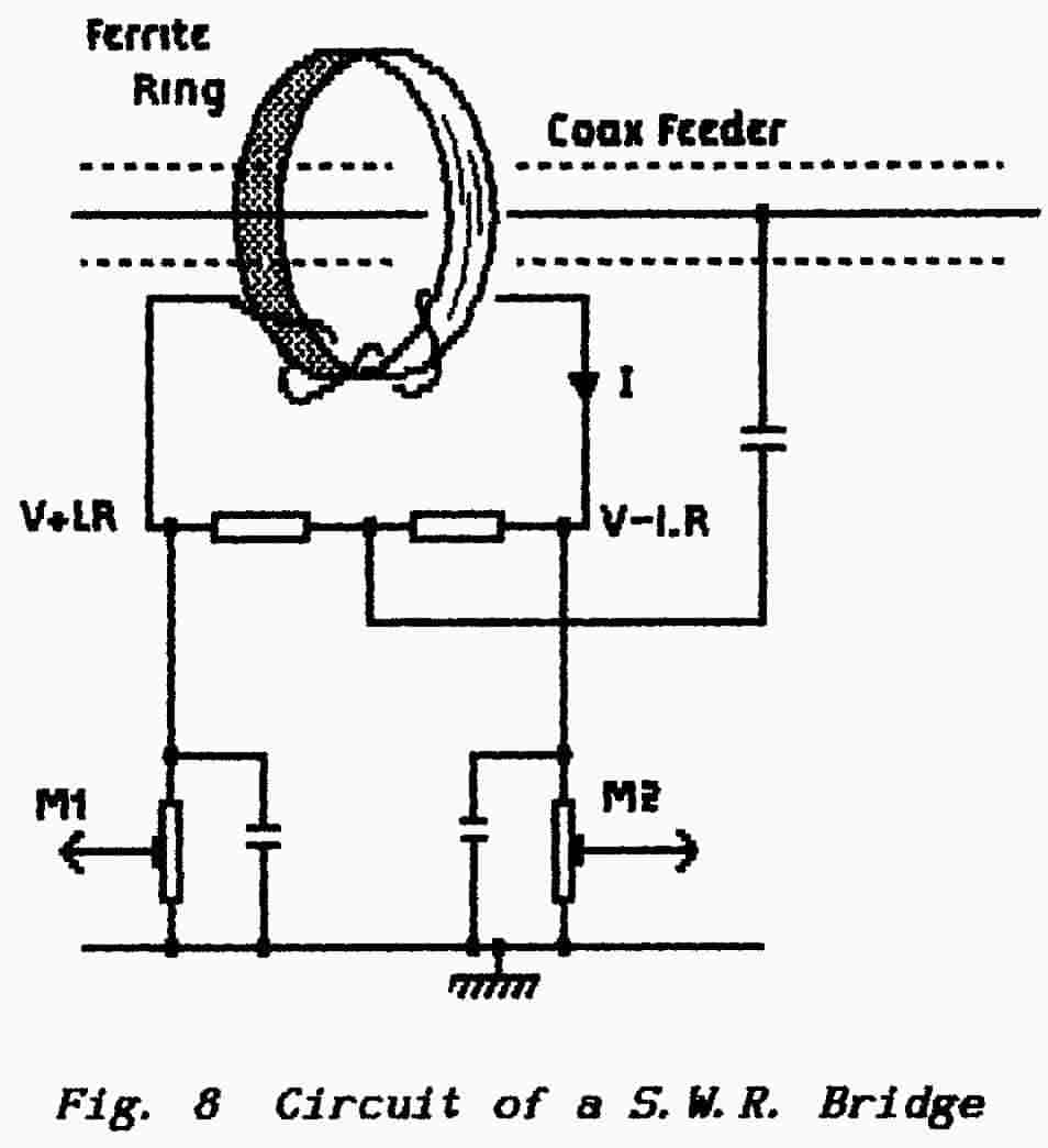 |
The current is sampled by means of a toroidal transformer as described under 1.10.5 in Lesson-5 of Fundamentals-1 . The resultant current is fed into two identical resistors ; this provides a centre-tap from which, at opposite ends of the transformer, two 1800 signals are available. The line voltage is sampled by simply tapping-off a proportion of the signal through a small capacitor. (A resistor can be used here but, not only does it dissipate some of the line-power, it must have considerable physical size to enable it to get rid of the heat generated within. ) Note however that, for a high-power meter, the capacitor must also be capable of carrying the current which results and also of withstanding the line voltage that will result should the feeder not be properly terminated when full power is applied. Two outputs are provided each one being a product of current and voltage but the two currents used are 1800 displaced. |
To set-up the circuit power is fed into the matched feeder, first in one direction and then in the other, and the appropriate variable-resistor is adjusted to achieve zero power indication. The device is often arranged with two meter-movements one of which has a right-hand zero. The scale is calibrated so that the pointer which moves to the right indicates the forward power and the pointer which moves from right to left indicates the reverse power. Where the two pointers cross a special scale indicates the standing-wave ratio.
In theory the device works equally in either direction. In practice however the "forward" circuit is desensitised so that the two meters give roughly equal indications over the normal operating range which makes possible the cross-pointer indication of swr. Thus a wrong connection of these instruments could result in damage.
In these devices for use below 30 MHz the toroidal transformer usually takes the form of a ferrite ring through which the centre conductor of a coax feeder is threaded. The secondary winding is a few turns threaded around the ferrite. Obviously the ferrite ring must be suitable for the frequencies to be used and it can operate only up to that power level where magnetic-saturation begins to occur.
Properly designed these instruments are not frequency-conscious and so they can be calibrated in terms of Absolute Power provided of course that bandwidth limitations are observed.
** For the R.A.E. you should be familiar with the formula which relates the degree of mismatch with the s.w.r. i.e.
s.w.r. = Vmax/Vmin = Imax/Imin = Zo/R
>>>>>>>>>>>>>>>>>>>> PAGE 18 <<<<<<<<<<<<<<<<<<<<
where Z0 is the characteristic-impedance of the feeder and R is the resistance of the load (the expression assumes some complication when the load is reactive). See also under 2.3.6 Standing Waves and SWR in Lesson-7 of Fundamentals-2.
The above methods of measuring power are suitable for continuous-wave emissions and, theoretically, for some forms of modulated waves, For example, the division of power between the carrier and the sidebands is known and so it is possible to make allowance for any modulation. There is a very real problem however in that the sideband power increases with the degree of modulation and so determination of the modulation index is necessary.
Power measurements with ssb transmissions cannot be made with these simple techniques because the output from a ssb transmitter is zero until modulation is applied. While the peak power could be measured by applying a continuous audio tone (a single audio frequency) few P.A. stages would survive such treatment for more than a few seconds. As with a.m. signals there is still the problem of determining the degree of modulation.
The oscilloscope gives a pictorial display
of waveform and enables these difficulties to be resolved. It can also be used
for straightforward measurements in place of a voltmeter (from dc up to the
maximum usable frequency of the oscilloscope), to measure waveform distortion
and to determine the modulation index.
The heart of an oscilloscope is the cathode-ray display tube which, in reality, is an overgrown valve. Its two main parts are the electron gun and the phosphor-coated screen which is sprayed on to the inner surface of an evacuated glass envelope.
The electron-gun is named because its purpose is to shoot a pencil-beam of electrons at the screen which glows at the point of impact. By moving the beam it is possible to trace diagrams on the screen. The glow lasts for only a short time after the beam has moved on and, by constantly rewriting the diagram, a moving display is formed. Use of long-persistence screens makes it possible for slow-moving or short-duration signals to be displayed but, of course, such tubes blur signals which change rapidly.
The gun consists of a heated cathode and a grid which, as in the triode valve described under 3.12.2 (Lesson-2 of Electronic Amplifiers), produces a controlled flow of electrons to an anode. In the electron gun however the anode has several parts often referred to as anode-1, anode-2 and anode-3 ; by varying the relative potentials on these components it is possible to focus the electrons into a fine beam.
>>>>>>>>>>>>>>>>>>>> PAGE 19 <<<<<<<<<<<<<<<<<<<<
The gun also possesses two pairs of plates, one pair positioned horizontally and one pair vertically between which the beam passes on its way to the screen. Voltages impressed between the plates of each pair cause the beam to bend and so change the position of the glowing spot seen on the screen. In line with mathematical convention horizontal movement of the spot is referred to as the X-direction and vertical movements as the Y-direction.
In most general usages the horizontal movement is used to indicate time and so the waveform which causes this deflection is referred to as the Timebase. Any signal which causes vertical deflection of the spot, in conjunction with the Timebase, forms a waveform trace across the screen which becomes a plot of voltage against time.
The screen has a transparent cover on which
is inscribed a graticule - a grid of squares - which facilitates measurements
on displayed waveforms. This is used in conjunction with calibrated controls.
Fig.9 shows the main features of an oscilloscope in block-diagram form. For the display tube the power-supplier produces a negative extra-high tension (e.h.t.) supply around 2-kV - which can be very unpleasant if not dangerous. The beam-deflection plates must be held at or close to the final anode potential if they are not to repel the electron-beam and so the vertical-deflection amplifier (the Y-anplifier or Y-amp) needs to deliver its output waveform relative to this potential. For both safety and convenience the input to the Y-amp must have one leg grounded or, at the very least, close to ground potential and so the tube is operated with the final anode at zero and the cathode taken to -2 kilovolts.

>>>>>>>>>>>>>>>>>>>> PAGE 20 <<<<<<<<<<<<<<<<<<<<
The filament (or heater) of the tube must be supplied from a separate well-insulated winding on the mains-transformer.
The e.h.t. is applied across a resistive potential-divider to obtain the various potentials required for the tube operation. Generally anode-1 & anode-3 are taken both to the full supply voltage but anode-2 to a variable resistor and this provides the Focus control. Anodes 1&3 are discs with a hole through which the electron beam passes while anode 2 is cylindrical. The lowermost resistor provides cathode bias for the gun and a variable-potential applied to the grid is the Brilliance control ; it sets the beam-current.
The Timebase Generator can be switched to be free-running (i.e. it oscillates) or to produce an X-deflection only when prodded or triggered. In either mode it may be fed with a Synchronising or triggering signal which ensures that it keeps in step with the applied waveform so as to produce a steady display. This trigger waveform is derived, either from the input waveform or from a separate External Trigger input, in a Trigger or Synchronising Amplifier.
The timebase waveform has a sawtooth shape that sweeps the spot steadily across the screen from left to right and then rapidly returns it to the left-hand starting position ready to start the next sweep. This waveform is fed to the X-amplifier which provides a facility to control the amplitude (the X-Gain Control) and also mixes it with a variable dc-signal which adjusts the position of the trace horizontally across the screen.
The waveform under test is applied to a Y-amplifier which provides a Y- Gain facility and also mixes in a second variable dc-signal which adjusts the position of the trace vertically across the screen. There is often another optional input to this amplifier in the form of a square-wave generator with a fixed amplitude which is used to calibrate the oscilloscope in the Y-direction thus facilitating accurate measurements.
There are many variations in oscilloscope design which depend largely on the major use for which the instrument is intended but, essentially, they all follow this basic layout.
The uses of an oscilloscope for measurements likely to be needed in an Amateur Station are given in the next Lesson.
END OF LESSON 3
>>>>>>>>>>>>>>>>>>>> PAGE 21 <<<<<<<<<<<<<<<<<<<<
QUESTIONS
1. State the the two methods of measuring c.w. power using a dummy load and rf-meter.
2. What problem arises in trying to measure power with this technique when the carrier is modulated ?
Why is this technique useless for ssb transmissions ?
3. In your own words describe the basic action of a reflectometer ; i. e. a directional-coupler or a s.w.r. bridge arrangement. (The R.A.E. does not require a detailed knowledge of their operation.)
4. In broad outline only what facility does an oscilloscope provide ?
Given that you have available only an oscilloscope with a 1-volt peak-to-peak squarewave calibration-waveform can you put together an experiment to check the emf of a battery believed to be 6-volts but encapsulated and with all labeling destroyed ?
6. RF power is to be measured using a dummy load and an oscilloscope as a voltmeter. So far in this Course we have not dealt with the difference between peak, average and R.M.S. values of a sinewave but can you suggest why measuring the peak-voltage of the carrier will not yield the correct power ?
>>>>>>>>>>>>>>>>>>>> PAGE 22 <<<<<<<<<<<<<<<<<<<<
Back to Top of PageAn oscilloscope can be used to make most of the measurements carried out by standard multimeters plus a few more which are difficult without the pictorial display. For some jobs the 'scope is perhaps a bit clumsy but it is capable of great accuracy.
The display tube is normally electrostatically deflected, which means that the trace responds to a voltage input, and so current measurements are not easy without introducing an impedance into the current path. Elderly valve-operated 'scopes may be found which are fitted with deflection coils to facilitate current measurements by magnetic deflection ; although it may be thought that such devices would be useful, with modern current-operated semiconductor devices the need to open the circuit for series-connection means that it is usually easier to make voltage measurements and to calculate the current.
Measurement of Direct Voltages
This is a simple matter with a 'scope. Although the timebase is not required it is best to allow it to run so that a straight line appears on the tube. A stationary spot left for some time is likely to damage the screen-phosphor.
With the 'scope input shorted the Y-shift control is adjusted to bring the line on to one of the graticule lines. The direct voltage to be measured is then connected and the new position of the line noted ; if the line goes off-screen or fails to move sufficiently then the Input Range selector must be set appropriately.
The screen graticule may now be calibrated
by using the internal calibration waveform or by applying a signal from a known
calibrated source (e.g. a Standard Cell as described in Fundamentals-1).
Measurement of Alternating Voltages
The basic technique for measuring the amplitude of an alternating signal is just the same but there are a couple of pitfalls. The timebase should be set so that several cycles are displayed which makes it much easier to set the waveform against the graticule lines.
The easiest parameter to measure is the peak-to-peak voltage ; i.e. from the most negative part of the waveform to the most positive part of the waveform. Indeed for irregular (non-sinusoidal) waveforms this is the only practical measurement. As shown in Part 7 however the average value for a sinewave between the two peaks (or crests) is zero and so this measurement is only a step on the way.
At the peaks of a sinewave the maximum value of the voltage will drive a maximum value of current through a resistive load and so produce a maximum value for the power which is being dissipated. Between the peaks the voltage is zero and power is not dissipated at all. We need to find a value, somewhere between these two, which represents the true power being dissipated: we are looking for that value which gives the average power that is dissipated over a complete cycle, the value that makes the heating effect of an alternating current the same as the heating effect for a direct current.
>>>>>>>>>>>>>>>>>>>> page 23 <<<<<<<<<<<<<<<<<<<<
Back to Top of PageThis value is known as the r.m.s.(root-mean-square) value of the waveform and it is derived for you in Part 7 of this Course ; for the R.A.E. you do not need to be able to derive this value but you must understand its meaning.
The peak (or crest) value is found by halving the peak-to-peak value; this is a more accurate method than trying to estimate the position of the zero line. From this measurement the RMS Value is obtained by dividing by root-2 (rough rule-of-thumb either multiply by 0.7 or divide by 1.4).
Peak-to-peak values are measured with an oscilloscope by comparing the waveform with the calibrated graticule or a calibrated Shift control; from this the R.M.S. value is found by calculation.
Measurement of Phase Difference
Because an oscilloscope draws a picture of the waveform it is not difficult to observe phase shifts provided that both waveforms can be displayed simultaneously. There are three ways to achieve this facility:
(a) The best and most expensive way is to equip the display tube with two separate guns.
(b) A single gun may be fitted with a beam-splitter plate which, after the beam has passed through the X-deflector plates, divides it into two separate parts each of which passes through its own Y-deflector plates.
(c) A single-gun tube is employed but an electronic switch alternates the display between the two input amplifiers and1 simultaneously, switches the shift potential to give the impression of a 2-gun display.
Switching can take place either during the flyback period between traces or by using a chopper technique in which the switching takes place at a relatively high frequency. Provided the switch operates with truly 'fast' transitions the interruption of the displayed waveform is not a problem.
Chopper techniques are particularly useful when observing slowly-changing waveforms because they eliminate the flicker caused by displaying each "trace" alternately.
With two traces displayed on the screen it is easy to observe any phase-difference but not so easy to make an accurate measurement. The
>>>>>>>>>>>>>>>>>>>> PAGE 24 <<<<<<<<<<<<<<<<<<<<
Back to Top of Pagetechnique used is illustrated in Fig. 10 . The time-base is adjusted so that
alternate sweeps are displaced by 1800 and each positive-going crest
is accompanied by a negative-going crest. The cross-over points give
an accurate position for the zero line and also are accurately separated by
1800.
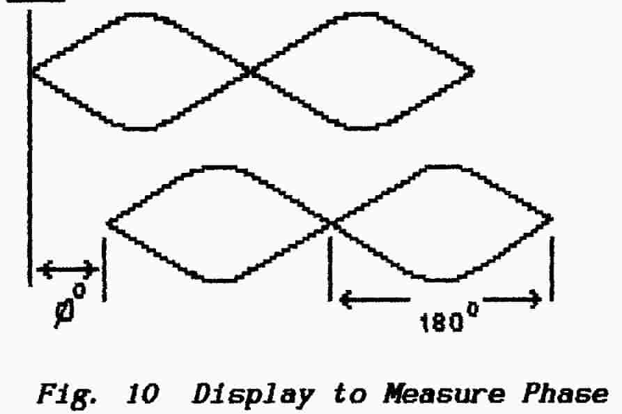 |
The distance between crossovers,
measured against the graticule (or with a small ruler), gives a value for
1800 and the displacement between cross-overs is measured in
the same units. A direct comparison of these two figures enables the phase-
shift to be calculated in degrees.
For such measurements to be successful it is necessary of course that the two input and amplifier circuits have very similar performances with regard to both frequency and phase ; i.e. they must produce identical signal-delays.
|
Measurement of Distortion
Small amounts of waveform distortion are not very noticeable on an oscilloscope trace below about 5% . In general there are three types of distortion which it is informative to recognise:
(a) Second-harmonic Distortion is characterised by a lop-sided waveform in which the "half-cycles" on one side of the zero-line have longer durations than the half-cycles on the other side(b) Third-harmonic distortion produces a balanced waveform with the successive half-cycles identical but characterised by flat or double-humped crests with too-steep skirts between
(c) Distortion produced by overloading a negative-feedback circuit is very distinctive because the rounded shapes are replaced by sharp spiky waveforms. Negative feedback does its best to cancel out distortions but, once the circuit has reached its limit, the failure of feedback control is spectacular and the onset of distortion is very sudden.
It is not far from true to say that there is little point in measuring distortions which are easily visible to the eye. Quantitive measurements are most useful when the distortion is small (the harmonic-amplitudes are relatively low) and when, of course, they are most difficult to detect.
For such measurements an oscilloscope is put into differential mode (often designated as Y1-Y2). The (hopefully-pure) waveform from the signal generator is fed also to one input of the 'scope ; the other input to the 'scope is connected to the output of the device under test. The two amplifiers are connected so that their outputs are 1800 out of phase and so tend to cancel. With suitable adjustment of gains those components which are present at both the input and output of the equipment under test
>>>>>>>>>>>>>>>>>>>> PAGE 25 <<<<<<<<<<<<<<<<<<<<
Back to Top of Pageare cancelled and so the only signal which is displayed is those small— amplitude components which are generated within the equipment namely the products of distortion. Because the main signal components have been eliminated it is now possible to raise the gain of the oscilloscope amplifier and so render the distortion more visible,
Once again however this trick is only successful if the two oscilloscope amplifiers have similar performances in both frequency and phase.
** Measurement of Modulation Depth
Few Amateurs work straightforward a.m. these days but you should be familiar at least with methods used to check modulation depth both with double-sideband signals and ssb signals. Should you under-modulate then the only problem is that your signal will be less successful in making contacts; over-modulation however produces spurious and illegal transmissions which can spread over a surprising amount of the spectrum.
With double-sideband amplitude-modulation the carrier amplitude is made to vary with the value of the modulating waveform ; over-modulation results in the carrier being interrupted for short periods at the (-ve) peaks of the modulating waveform.
Fig. 11 shows in diagram (a) the normal representation of an amplitude modulated carrier with low-level modulation, in diagram (b) the same carrier with 100% modulation and, in diagram (c) the result of over-modulation. To measure the depth of modulation the maximum and minimum amplitudes of the carrier are required as described in Fig. 4, Lesson 2 of Fundamentals 2.
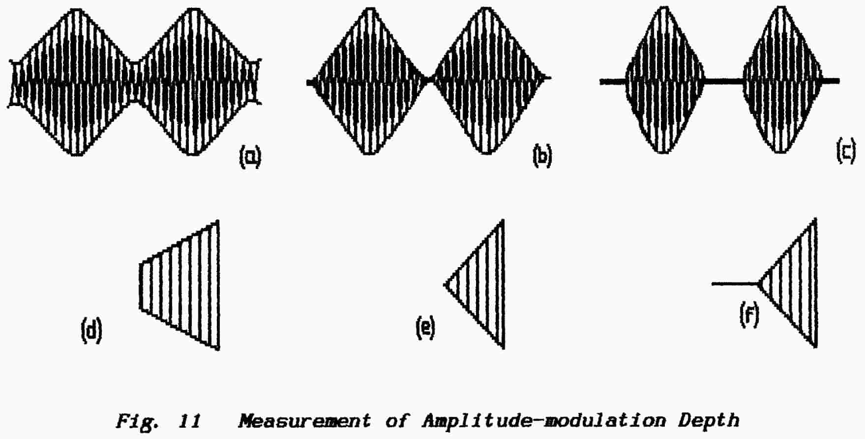
The most accurate way to make this measurement is shown in diagrams (d, e, f). Here the timebase has been switched-off and the X-amplifier is driven with the modulating waveform. As the modulation increases from (say) negative-peak to positive-peak so the trace moves from left to right across the face of the tube ; at the same time the modulated carrier increases from a minimum value to a maximum value.
>>>>>>>>>>>>>>>>>>>> PAGE 26 <<<<<<<<<<<<<<<<<<<<
This action is reversed during the following half-cycle of the modulating waveform. The display should be straight-edged and trapezium shaped as shown ; variations from this form are evidence of distortion.
** Measurement of Power with S.S.B.
A single-sideband transmission consists of
side-frequencies only and so
(a) a signal is present only when modulation is applied
(b) signal level is determined by modulation amplitude.
The term modulation index has little meaning.
The only practical way to measure a s.s.b. signal is to determine the maximum power-level known as the peak envelope power or p.e.p. Such a measurement has two possible purposes:
(i) to determine the performance of a P.A. stage
(ii) to control the signal-level that is being radiated.
To measure the first of these it is necessary (in theory) only to increase the modulation amplitude until a limiting condition is achieved. However, in use, a P.A. produces maximum output intermittently mainly as a result of speech explosives (such as the letters t,d,k,p) and so it is uneconomical to build a P.A. stage which is capable of delivering its maximum output continuously. Thus the above power-measuring technique would destroy the equipment.
Short-duration peaks of power can be measured by use of a slugged meter; this is arranged with a shunt capacitor and a diode to have a fast charging-time but a slow discharging-time . Although such a meter tends to dwell on the peaks it is not a very accurate method for very short pulses of power such as are encountered in speech waveforms.
To obtain a modulation waveform which will deliver short-duration peaks in a controlled fashion a two-tone oscillator is used. The outputs from two separate audio oscillators are combined to produce a beat ; when their amplitudes are adjusted to the same level the beating signal has the appearance of a 100%-modulated carrier in that the amplitude varies from zero to twice the amplitude of either.
Fed into an s.s.b. transmitter this produces a sideband signal which beats in the form shown in Fig. 12(see also Lesson-5 in Fundamentals-2)
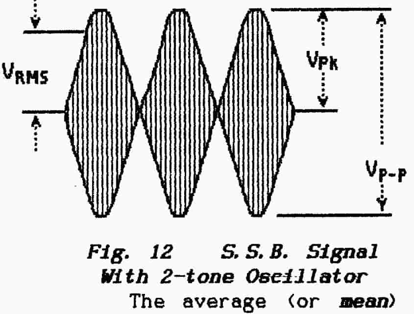 |
This rf waveform can be displayed on an oscilloscope connected
across a dummy load and the peak-to-peak voltage determined. From this
the p.e.p can be calculated using the value of the dummy load ; the maximum
value of the peak-to-peak voltage (V in the diagram) is first halved to
obtain the peak voltage, multiplied by 0.707 to obtain the R.M.S. value,
squared and then divided by the resistance of the dummy load (E2/R).
The average (or mean) power is less than the peak power; for a |
>>>>>>>>>>>>>>>>>>>> PAGE 27 <<<<<<<<<<<<<<<<<<<<
Back to Top of Pagereasonably symmetrical waveform it could be expected to be around 50% of the peak power but it depends entirely on the waveform of the modulating signal. It is the mean power for which the transmitter is designed; although the design permits this figure to be exceeded for brief periods any prolonged output at peak power must cause overheating and destruction of the P.A.
The mean power can be measured by inserting an r. f. ammeter in series with the dummy load ; the meter must of course be usable at the carrier frequency in use and must give its indication in terms of R.M.S. values. Such a meter is often incorporated into dummy loads and it is calibrated in terms of power.
These measurements cannot be undertaken when the modulation is a speech waveform and it is for this reason that the Licence conditions specify a maximum permitted p. e. p. ; if the limits of the 2-tone envelope are noted on the oscilloscope display when the output is set to 400 watts p.e.p. then the modulation controls of the transmitter can be set so that, when speaking into the microphone, the transmitted peaks do not exceed the permitted maximum level as marked on the oscilloscope screen.
Lissajous Figures
These provide a simple but useful technique for measuring the parameters of a sinewave. The figures are formed by switching-off the timebase and feeding the horizontal (X-deflection) amplifier with a known sinewave derived, for example, from a signal generator ; the Y-amplifier is fed with the signal under test.
To start, suppose that the X-deflection and the Y-deflection are exactly similar waveforms. As the waveform voltage shifts from max-negative to max-positive so the spot on the oscilloscope tube will travel from left to right and also from bottom to top. During the following half-cycle the spot will retrace its steps exactly. The result is a straight line sloping upwards and to the right. If the two waveforms are of equal amplitude then this line will lie exactly at 45o.
If the Y-deflection waveform has a frequency twice that of the X-deflection waveform then, while the spot is moving from left to right, it will move also from bottom to top and then back to the bottom again. The result is a bent line. During the next half-cycle of the X-waveform the spot will repeat its up-and-down motion to draw another bent line on top of the first trace. Any phase-shift present will cause the bent line to open out into a loop and the display appears as two "sinewaves' forming a ring.
If the Y-deflection waveform has a frequency three times that of the Xdeflection the ring will show three complete cycles. If the Y-waveform is not an exact multiple of the X-waveform then the displayed figure will constantly rotate like a circle of children playing ring-of-roses.
Thus, to measure frequency accurately (or, at least, as accurately as the calibration of your signal generator), the timebase is replaced by the signal generator and the frequency is altered until the Lissajous figure becomes stationary. The number of complete cycles displayed on the figure shows the harmonic relation between the signal under test and the signal-generator output.
>>>>>>>>>>>>>>>>>>>> PAGE 28 <<<<<<<<<<<<<<<<<<<<
Back to Top of PageComponent Testing
An oscilloscope can provide a very useful way to test components without removing them from circuit. Bear in mind however that all measurements may need to be interpreted arid not taken at face value. For example, a resistor may give a test result that claims it is a diode. This may mean that the resistor has become open-circuit and the equipment is measuring a diode via a shunt path ; OR it may mean that the resistor has a very high value compared with the reverse resistance of the diode and so the equipment is "seeing" only the diode. The answer lies in the circuit diagram and it may eventually be necessary to remove the component from the circuit for testing.
This test circuit is a development from the Lissajous-figure technique described above. Similar waveforms are fed to the X and Y amplifiers but that to the Y-amp goes via the test-prods. When a resistor is connected the result is a straight but angled line as described above. When the test prods are open-circuit the Y-deflection becomes zero and so a high-resistance appears as a horizontal line. Similarly a very low resistance appears as a vertical line.
As the applied voltage is increased so a diode at first pretends to be an insulator but then abruptly changes its mind and becomes a low-resistance. Consequently the display switches abruptly from horizontal to vertical (assuming that the diode is still a diode!).
The exact form of the display depends on the test circuit, on the setting of the gain controls and on the nature of the item under test.
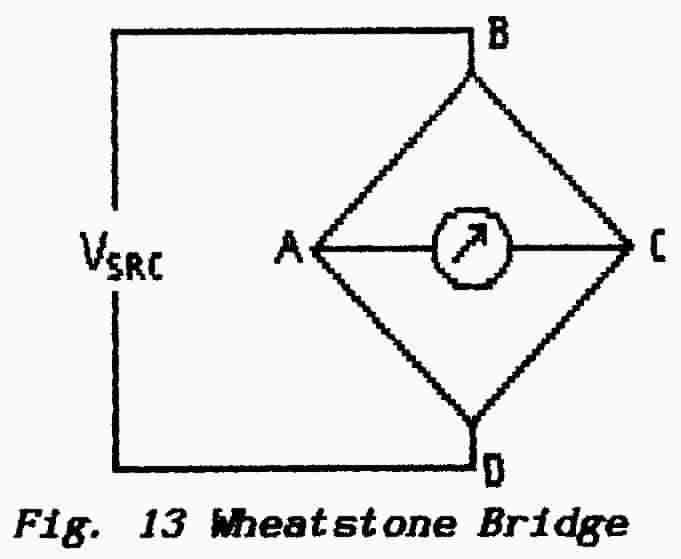 |
The basic Bridge circuit, shown
in Fig. 13, is the Wheatstone Bridge. This consists
of four resistors connected as two series pairs in parallel across a source.
The source can be either dc or ac but, for accurate measurement, dc is
the more usual because it eliminates the effects of reactances.
In its simplest form the Bridge consists of four equal resistors each of which must draw equal currents ; it follows that the p.d. across each is half the source voltage. Under these conditions the potential at point A is exactly the same as the potential at point C and so a meter connected between A and C shows zero deflection.
|
The value of an unknown resistor can be determined from this arrangement ; resistor BC is made variable with a calibrated scale while resistor CD is replaced by a pair of terminals to which the unknown resistor is connected.
>>>>>>>>>>>>>>>>>>>> PAGE 29 <<<<<<<<<<<<<<<<<<<<
Back to Top of PageResistor BC is then varied until the meter-deflection is zero when, as described above, the value of BC (read from its calibrated scale) is the same as that of the unknown.
The range of the Bridge can be increased by using different ratios between resistors BA and AD ; in general the equality BA/AD = BC/CD will always result in zero deflection of the meter.
The basic Wheatstone Bridge can be re-arranged in a variety of ways using inductors and/or capacitors with resistors, together with an ac source, to measure reactances. Sometimes the ratio arms BA and AD take the form of a tapped secondary winding on a transformer through which the ac-source voltage is fed. Dependent on the arrangement of the reactances the bridge may be balanced by either a series combination of R+X or by a parallel arrangement of R & X thus yielding the phase conditions as either an impedance or an admittance (see Lessons 7, 8 & 9 in Fundamentals-1).
Knowledge of bridges and bridge measurements is not required for the R.A.E. but you may be puzzled by references in the literature to Noise Bridges. It is an unfortunate name because it does not refer to a bridge arrangement intended to measure noise ; it is a bridge arrangement meant to measure L, C & R but which uses a noise-source as the ac source mentioned above. Instead of using a meter to indicate the balance point the Operator listens to "white noise" on headphones and determines balance by a dip in that noise level.
However, there is a point that I would raise here and that is the importance of the quality of signal generator which is used to drive the bridge. When a Bridge has been balanced, and the output (either on a meter or on headphones) is at its minimum, the balanced condition applies only to the fundamental of the Bridge-oscillator; any harmonics present in the waveform will break-through the Bridge because, at that frequency(ies) the Bridge is NOT balanced. Hence when starting to set-up a measurement the Bridge-oscillator must be set to its lowest possible output and the Bridge-detector (which feeds either a meter or headphones) should be set to maximum gain. As the balanced condition is approached so the detector gain is turned down and the oscillator output increased. A low-quality signal source with a rich complement of harmonics is useless for Bridge work.
END OF LESSON 4
* * * * * * * * * * *
QUESTIONS
1. A sinewave is displayed on an oscilloscope screen with a peak-to-peak waveform that occupies the space between four 1-cm graticule squares. Given that the Y-gain controls are set to "5OO mV per cm" what is the R.M.S. value of the waveform ?
2. The above waveform is being developed across a 50-ohm dummy load. What power is being delivered by the source ?
3. Why is power measurement difficult in s.s.b. equipment ?
How would you use an oscilloscope display to set the limiting circuits(probably a so-called speech processor) so that you did not exceed the Licensed limit of 400 watts p.e.p. ?
4. A transmitter output is fed to a dummy load across which an oscilloscope is connected. The transmitter is operating in the a.m. mode with a modulation waveform which is fed also to the X-deflection of the oscilloscope.
In the trapezium-shaped display the maximum height is 2½ cm and the minimum height is ½-cm. What is the depth of modulation ?
>>>>>>>>>>>>>>>>>>>> PAGE 30 <<<<<<<<<<<<<<<<<<<
This rather curious title is usually shortened to the letters E.M.C. and it refers to the twin matters of causing interference to other users of the radio spectrum and to receiving interference from other users.
The basic idea seems to be that all electrical/electronic equipment should be compatible with the electrical environment ; I cannot say that it enlightens me however.
Many of the most common and obvious causes of being a nuisance to other users have been mentioned already in previous Sections of this Course:
(i) Harmonic generation caused by overdriving, wrong bias or other faults in transmitter adjustment
(ii) Harmonic generation caused by bad keying technique - see key-click filter.
(iii) Excessive side-frequency generation through over-modulation or because the microphone audio circuits are generating harmonics of the modulating waveform ; see speech processor.
(iv) Harmonic radiation from the Drive
(v) Spurious oscillations caused by wrong adjustment of the transmitter or because the apparatus lacks sufficient margin of stability and it bursts into oscillation on modulation peaks
(vi) Intermodulation products which are the result of beats between two signals which may be either legitimate signals or unintentional products as listed above.
(vii) RF radiation from computer-type equipment
(viii) Waveform distortion imposed on the mains from the modern habit of generating dc supplies without the use of a smoothing choke. The very-large values of capacitance involved result in very-large but short-duration spikes of current being drawn from the mains at the peak of each cycle. The high-order harmonics generated are radiated from the mains wiring . It is now illegal to design or to supply such power units.
In general the "cure" for all the transmitter problems is a suitable low-pass filter but it must be emphasised that such filters are placed at the output of transmitters as (a) a precaution (b) as a final clean-up of an otherwise good signal. It is very bad practice to be sloppy about adjusting a transmitter and then (hopefully) to rely on a l.p.f. to reduce the resulting mess.
>>>>>>>>>>>>>>>>>>>> PAGE 31 <<<<<<<<<<<<<<<<<<<<
Back to Top of Page** As a cure for problems of the type in (v) above you may often see a small-value resistor (around 100 to 200 ohms) connected in series with the collector of a transistor (or the anode of a valve) P.A. stage. The resistor or perhaps a small choke is mounted as close to the active device as possible. Such a resistor is referred to as a stopper (anode-stopper, grid-stopper, collector-stopper) and is a likely subject for a question in the R.A.E. Each electrode of a valve or transistor has a (stray) capacitance to the others and the stopper resistor is in series with that capacitance and so forms a low-pass filter.
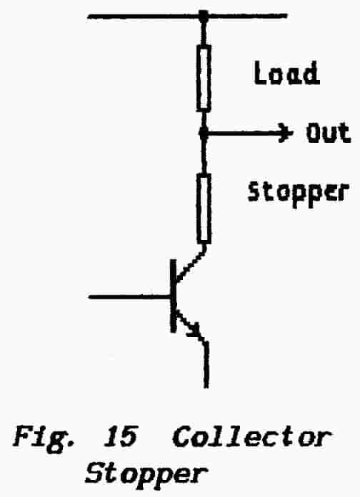 |
** The stopper must have an impedance which is low in comparison with the load at the operating frequency but which is greater than the inter-electrode reactance at the parasitic frequency. It is not uncommon to see a stopper in the form of a small choke wound over a resistor thus forming a lossy (or low-Q) choke whose function is to both stop and dissipate spurious signals - compare this with the use of a ferrite bead as mentioned in 6.6.2 below. [With reference to the Lesson on oscillators it should be noted that the addition of resistance (loss) to a resonant circuit can ensure that the Q is too low for oscillation to take place.] As mentioned in Part-2 a low-pass filter cannot cure all ailments. Distortion in the modulating-signal chain will produce unwanted side-frequencies both above and below the carrier frequency. The final l.p.f. will remove the out-of-band upper side-frequencies but it will ignore the lower side-frequencies. |
A bandpass filter will, of course, take care of this situation but, apart from being an expensive and unnecessary cure, it represents a sloppy approach that is likely to land an Operator in more trouble than he reckoned
Unfortunately it is possible to cause severe interference even when the transmitted signal is immaculate. Where this is the fault of the Amateur Operator he must, of course, take steps to eliminate the nuisance ; where it is not his fault he is not liable but, if you wish to live at peace with your neighbours, a courteous and helpful attitude is to be recommended.
Many receivers use an intermediate-frequency around 10.7 MHz which is the third-harmonic of carriers in use on the amateur 3.5 — 3.8 MHz band. When close to a transmitting aerial the strong inductive-field is very likely to find its way into the if-amplifier and so give rise to a complaint that " ... you are coming in all round the dial ... " ; in fact, of course, the interference is not coming through the tunable front-end at all. The carrier may be immaculate, the keying waveform perfect and the transmission is not in any way spreading itself across the spectrum. The fault lies in using an unscreened receiver too close to a transmitting aerial. That one is very difficult indeed to explain to a non-technical and irate neighbour.
Harmonics can be generated in a parasitic circuit which contains a nonlinearity — i.e. a partial or low-grade rectifier. This could take the form of a rusty joint or bolt in local metalwork, a corroded joint in plumbing, a badly made or corroded connection in household wiring. The offending "circuit" is excited by radiation from the transmitter aerial, generates harmonics through its non-linear element and then re-radiates the degraded signal. Such a parasitic circuit may not be at all easy to locate.
>>>>>>>>>>>>>>>>>>>> PAGE 32 <<<<<<<<<<<<<<<<<<<<
Back to Top of PageSometimes household wiring or plumbing can form a closed loop which just happens to resonate within one of the amateur bands ; the result can be a large circulating current with any sort of interesting effect. The problem here is to first locate that loop and then to add a reactance to detune it.
Non-linear elements are to be found in all household electronic equipments in the form of transistors or similar semiconductor devices. If the signal radiated from a transmitter aerial gets into a television receiver, a video-recorder or any form of audio equipment then it is likely to be demodulated and the result becomes a permanent part of the signal which the equipment is supposed to be processing. It can even appear in the telephone
The only practical cure for this type of problem, apart from reducing power, is to re-site the aerial and/or investigate its design to ensure that the signal is radiated into space and is not irradiating the neighbour's (or your own) household.
The field-strength (signal strength) laid down by an aerial is proportional to the square-root of the radiated power and so it might appear that power levels do not have much effect on interference. In practice however it is found that power reductions can have a marked effect and it is good practice never to use more power than is required for the Contact of the moment.
** Marks can be picked up in the R.A.E. by calculating field-strength from a simplified formula:
e = 7√erp/d
where e is the signal strength in Volts-per-metre (V/m), erp is in watts (estimated radiated power) and d (in metres) is the distance from the aerial to the point in question. However it is difficult to see much practical use for the calculation.
It is said that the formula can be used to
give an idea of the probable field strength at the point where interference
is being caused by an amateur transmission. At the close range at which such
incidents take place it is likely that the close-in inductive field has more
to do with the problem than the long-distance radiation field with which the
formula deals. In any event it is difficult to see the benefit of the calculation
when trying to suppress such interference.
There is not a real set of rules for dealing with incoming interference. The important thing is to know the tools that are available and the techniques for which they have been formulated. In general the idea is to divert unwanted interference-currents away from the signal path and to divert unwanted voltages to ground. Mostly the techniques used to prevent unwanted radiations can be adapted to deal with unwanted incoming signals (irradiations).
>>>>>>>>>>>>>>>>>>>> PAGE 33 <<<<<<<<<<<<<<<<<<<<
By way of illustration Fig. 16 shows a small
brush motor such as may be found driving an electric typewriter or a sewing
machine. The circle represents the rotating armature and the two sloping lines
represent the "brushes" which carry power to that armature. Sparks
which occur at the brushes may cause radiation directly but they also cause
noise signals to flow into the supply cable which then acts both as a transmission
line and an aerial.
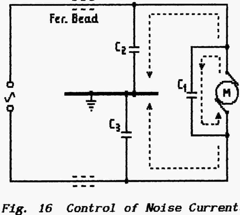 |
As shown these are of two types: |
The first of these can be confined to the motor by connecting a suitable small capacitor across the brushes (C1 in Fig. 16). The second type are diverted to ground or to the metal casing of the motor (C2 & C3) from which they complete their circuit by capacitive coupling to the armature. The three capacitors can be obtained built into a single unit with three connections which is known as a delta capacitor because of its resemblance to the Greek (triangular) symbol delta.
That a low-impedance capacitive path has been provided does not necessarily mean that the intended currents will take that path. Current will divide between the cable and capacitive paths according to their relative impedances thus, to encourage most of the current to take the capacitive paths, it is necessary to increase the impedance of the cable at the frequencies of the interference signals.
As shown in Fig. 16 small chokes are added in series with each leg of the cable. These may be bought off-the-shelf or hand-wound on small ferrite cores ; their small inductance presents little opposition to the flow of 50-Hz mains current but virtually open-circuits the cable to radiating frequencies.
As an alternative small ferrite beads are available which can be slipped over the wire. They come in different grades but, basically, these increase the line inductance ; they also add some loss to the circuit and so dissipate the unwanted energy.
As shown the choke/capacitor combinations keep unwanted interference currents within the device which is generating them. However, to protect that device against intruding currents driven into the mains by some other piece of badly-protected equipment, the chokes must be placed on the other side of the capacitors; i.e. between the capacitors and the device. A general-purpose filter unit can be made, which will keep rf currents both within and without the device, by placing a capacitor on each side of the chokes. Such a filter may be referred to as a pi-filter because of its resemblance to the Greek letter π.
>>>>>>>>>>>>>>>>>>>> PAGE 34 <<<<<<<<<<<<<<<<<<<<
With reference to Fundaznentals-2, Lesson-5 the above pi-filter is a low-pass filter . At high frequencies the choke open-circuits the signal path while the capacitors short-circuit that path to ground. At low frequencies neither the choke nor the capacitors are effective.
This filter is converted to a high-pass configuration by interchanging the positions of its components ; i.e. the series path is interrupted by a capacitor and the choke(s) is put in shunt to ground.
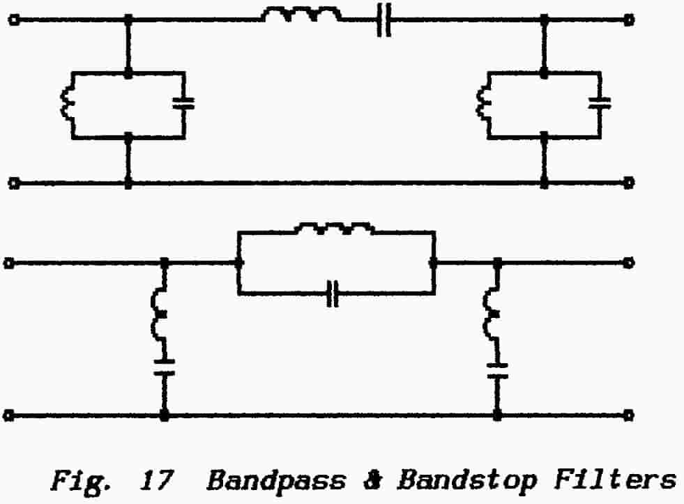 |
Both configurations can be developed by resonating the elements as shown in Fig. 17to form either bandpass or bandstop (trap) filters. The bandpass circuit can be useful in preventing the escape of unwanted signals while the bandstop can be useful in permitting the passage of wanted signals (such as your neighbour' s television service) while stopping the intrusion of your amateur transmissions. |
For the R.A.E. you are not required to design such filters but it is perhaps worth understanding their limitations. In the lpf, for example, the series choke is shunted by stray capacitances which set an upper limit to its effectiveness as an inductance. In a similar manner the shunt capacitors exhibit a small amount of inductance which sets an upper limit to their effectiveness as capacitors.
Indeed this is the situation illustrated in Fig. 17 where the reactors have been deliberately resonated. It follows that all chokes and all capacitors have limited capability set by their own natural resonance frequencies. Above their individual resonance-frequencies an inductor becomes a capacitor and a capacitor becomes an inductor. As frequency is increased the only cure for this is to reduce the value of the component but, again, there is a physical limit. Fortunately the reduced value of the component is compensated, in terms of reactance, by the increased frequency.
The coaxial feeder which connects a television receiver to its chimney-top aerial is often some 30 to 50 feet in length (say 10 to 15 metres) which means that it can act as a reasonably efficient receiving aerial which is λ/2 in length for the amateur 20 and 30 metre bands or λ/4 in length for the lower-frequency amateur bands. Earthing the braid of the coax at the television receiver merely turns this into a more efficient hf aerial .
>>>>>>>>>>>>>>>>>>>> PAGE 35 <<<<<<<<<<<<<<<<<<<<
For a nearby transmitter putting out some 100 watts or more there is likely to be a considerable current flowing on the tv feeder and it is not surprising if this appears in the internal circuitry and finally on the picture and/or the sound channels.
[As a matter of interest this was a serious problem when the first television transmissions took place from Alexandra Palace just before WW II. From ground to the top of the television-transmitter mast was almost exactly a quarter-wave at the frequencies of the medium-wave broadcast service from nearby Brookmans Park. As a result the broadcast services insisted on their rightful place in every camera and every piece of equipment used in the studio and their exclusion was a major headache. ]
An obvious cure is to disconnect the braid from the receiver but this has two unfortunate effects
(i) the television signal is attenuated as well as the hf interference
(ii) the inner, no longer screened, takes over as the vertical receiving aerial with possibly worse results.
One trick might be to break the braid and then bridge the gap with a small capacitor which will act as a somewhat crude high-pass filter. There is a possible danger however in that the amateur transmission could induce high voltages on the now unearthed coax feeder ; apart from tickling-up the family this voltage would then be capacitively-coupled onto the inner conductor and so re-appear at the receiver input.
The so-called braid-breaker arrangement threads the coax television feeder through a ferrite ring ; the turns should be well spaced and the first and last turns not permitted to come too close (to avoid the bypassing effect of stray capacitance). In terms of the outer braid this generates a small inductance which effectively open-circuits the braid and so interrupts the flow of the interfering hf currents.
Why does the inductance not stop the uhf television carriers (around 500-MHz) also ? In Lesson-8 of Fundarnentals-2 it was shown that the energy conveyed by a coaxial transmission line was carried by the electric and magnetic fields which are set up between the inner and outer conductors. The outer conductor screens the inner and so, when the feeder is coiled, the uhf magnetic fields of the individual coils do not add together. The transmission path may become a bit giddy but an inductive effect is not generated. You may prefer to think of it as cancellation between the current which flows on the inner conductor and current in the reverse direction which flows on the inside surface of the outer ; the interfering hf current flows only on the outer surface of the outer conductor.
Although it is affectionately called a braid-breaker the technique is not limited to coaxial cables. It can be very effective in reducing the flow of unwanted currents on mains cables by winding the cable onto a ferrite ring in exactly the same manner. It is perhaps more effective to use a properly-wound balanced choke in which the two legs of the circuit are married and wound together on a core ; the magnetic fields of wanted push-pull currents cancel and so do not generate an inductive effect while unwanted push-push currents aid in setting up a magnetic field.
>>>>>>>>>>>>>>>>>>>> PAGE 36 <<<<<<<<<<<<<<<<<<<<
Back to Top of PageTo get an hf aerial to radiate efficiently it is essential to provide a good low-resistance earth connection. A good earth connection is essential also to the techniques described above of screening and filtering to avoid problems with e.m.c. It is unfortunately true that a good low-resistance earth, if improperly used, can result in a fire and also in death by electrocution.
Power is generated and distributed as a three-phase supply. Essentially this consists of three wires each of which carries a 50-Hz waveform which is 1200 shifted in phase with reference to the other two. If power is drawn equally from all three wires the system is self- sufficient but, if the load is unbalanced, then a fourth wire is necessary to carry an out-of-balance current ; this is referred to as the neutral wire. The normal domestic single-phase feed consists of one of the phase-wires and the neutral which, nominally at least, is at earth potential.
It is unlikely that the neutral will be exactly at zero potential because of the volt-drop along its length caused by the current which flows on the wire ; this could be several hundred amps when a single feed serves several establishments.
Before the 1960's the house would have been supplied also with an Earth connection which usually consisted of the metallic sheathing of the supply cable. The actual connection to earth was made at the sub-station and it may not have provided a very good earth.
The danger was in the possibility of a break in the neutral line with the live 240-volt line still operative. This would leave all the equipment beyond the break at 240-volts even though it was no longer working. For this reason all electrical equipment was housed in metal casings which were bonded to the earth connection. A fault would not become a hazard as long as the metal casing remained efficiently earthed and a would-be repairer did not attempt to disconnect that earth. Hopefully any fault current flowing to earth via the casing would rupture a fuse and so disconnect the faulty equipment but that presupposed that a handyman had not rigged the fuse.
In a p.m.e. (protective multiple earth) distribution a separate earth connection is not supplied and the neutral conductor is bonded to earth wherever it may be convenient . This multiple earthing produces a lower-resistance earth and so greater safety. Such earthing takes place at each distribution point by bonding the neutral to gas and water supply pipes. A problem today is that much plumbing is carried out using plastic pipes and, even on older installations, plastic pipes may be introduced. This does not help with earthing problems particularly when a plumber cuts-out or uncouples a piece of steel or copper pipe and finds himself providing the earth continuity for a piece of faulty equipment.
All bondings to such plumbing must be made at the point where the pipe(s) enters the house so that it is not possible to interrupt the earth connection.
Hazards such as these are taken care of by a residual-current-device which essentially compares the current flowing in the live lead with that returning through the neutral lead ; the two currents should be identical.
>>>>>>>>>>>>>>>>>>>> PAGE 37 <<<<<<<<<<<<<<<<<<<<
An insulation fault will allow current to escape from the circuit and flow to earth (via the plumber ?). The r.c.d. uses a balanced transformer to detect any difference in the two currents and, for household use, it trips a circuit-breaker when this residual-current reaches 30 mA. It should perform this feat within a matter of milliseconds and so prevent any frying incidents.
The system works very well unless a keen amateur-radio enthusiast wants to add a separate earth connection to improve the radio-frequency performance of his system. It doesn't matter at all as long as
(a) faulty equipment is not present and
(b) the neutral connection to the house does not become disconnected.
This may not be a serious hazard for a town dweller until the Council decide to dig-up the road but, in country areas where overhead distribution cables are commonly used, it is not at all impossible.
With the neutral interrupted the amateur's rf-earth takes its place and the mains lead to the amateur equipment takes over as the earthed return for every establishment connected to that section of line beyond the break. A normal 5-amp mains lead is not intended to carry the several hundred amps of mains current that could be flowing along the neutral and so it will melt and start a fire. Should such an accident occur while the rig is being operated the Operator then takes over as the earthed return with dire consequences.
The best solution is to disconnect the mains-earth from the amateur equipment and also from every piece of equipment within 6-ft of the operating position (i.e. within reaching distance). All metal parts within that area must be bonded together and taken to the rf earth. Portable equipment, such as kettles, coffee pots, heaters, soldering irons must not be brought into the protected area unless plugged into a socket whose earth pin also goes only to the rf earth. [Note that all other fixed metal objects in the house should also be bonded together and taken to the incoming neutral/earth thus ensuring that, in the event of losing the neutral, everything floats at the same (240-volt) potential.]
It is essential that the power fed to this protected radio area be taken through a separate r.c.d. ; it is possible to obtain a wall socket with built-in r.c.d. or a plug-in type but take note of the current-limitations of the device you use. Do NOT disconnect your mains earth until an r.c.d. is in place.
There is a good article on this subject published in the R.S.G.B.'s RadCom in June 1987 under the title The Killing Ground.
>>>>>>>>>>>>>>>>>>>> PAGE 38 <<<<<<<<<<<<<<<<<<<<
END OF LESSON 5
* * * * * * * * * * * *
QUESTIONS
1. Why should you not rely on a low-pass filter at the output of your transmitter ?
2. What is a "collector-stopper" ?
3. Your neighbour complains that, when you were calling "CQ" a few minutes ago, you came out of his f.m. radio all over the band. What is the probable cause and what would you do about it ?
4. Some time ago our receiver, connected to the long-wire aerial, was producing a series of clicks or "crashes". These disappeared when the aerial was disconnected but were noticeably more frequent during gusts of wind.
An inspection of the aerial revealed that the end of a short length of chain, which was part of an upper stay for the mast, was swinging freely in the wind and constantly touching a lower stay-wire. The chain was tied-off with a piece of string and this completely cured the fault. Can you explain this ?
5. What are the basic techniques used when trying to eliminate interfering signals ?
6. What is a "band-stop" filter ? How might you use it ?
7. A good transmitter installation requires a good low-resistance earth. What is the source of the hazard such an earth can cause if you are fed mains power from a P.M.E. distribution system ?
END OF PART 6