BASIC RADIO THEORY
Fundamentals-1 dealt with basic Physics: this second Part of Fundamentals deals with basic aspects of Radio Engineering. Radio is a word which originated in America and which now replaces the original English word "wireless"; it refers to the transmission of information between two points without the use of connecting wires.
There is of course nothing new in transmitting messages over long distances; some of the early mechanisms include runners, horse-riders, drums, pigeons, semaphore machines, fire, smoke and the heliograph but the discovery of electricity brought the electric Telegraph. Two or more stations were connected by a pair of continuous conductors and, by means of a Telegraph Key, current was switched on and off according to an agreed code. With each change of current a Telegraph Sounder emitted a click.
The problems of the Telegraph were mainly that messages could be passed only between those stations which were connected by wires and those wires were vulnerable both to the weather and to accidents or sabotage. Marconi's famous experiments with electromagnetic (e-m) waves opened the way to world-wide communication because connecting wires were no longer necessary.
Marconi did not invent radio but built on the theoretical work of the physicist James Clerk Maxwell who first predicted the possibility of e-m waves. That such waves can exist is one thing; to use them for practical communication required a whole new technology to create such waves and then to utilise them.
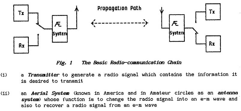
** A radio communication chain requires four separate parts (see Fig. 1)
>>>>>>>>>>>>>>>>>>>> PAGE 2 <<<<<<<<<<<<<<<<<<<<
(iii) a propagation path over which the e-m wave travels from the sending position to the intended reception point. This is the least reliable part of a radio-communication chain and it is an unfortunate fact that radio techniques do not automatically provide communication between two selected points
(iv) a Receiver whose function is to select the required signal from the many which an aerial system picks up, to amplify that selected signal and then to recover from it the information.
A Transmitter is an electrical ac-generator which is designed specifically to excite an aerial system into radiating an e-m wave. It is possible to connect a microphone-amplifier combination directly to an aerial but the resulting range of communication is limited to a few feet only. One exception to this is the Induction-loop which provides communication at audio frequencies with any point which is enclosed by the loop. This type of communication however is limited to one-channel operation because it is not possible to separate two or more signals.
** For e-m waves to propagate over reasonable distances it is necessary to use frequencies which are above the audio range ; however, efficient aerial systems are impossibly large until the frequency rises above several hundred kilohertz. Each communication channel is allocated a specific frequency and so it becomes possible to separate and to identify them (see under 1.13: Resonance).
** The information to be passed through each communication channel is impressed on that channel's individual radiation which, because it "carries" the information, is known as a carrier wave or simply as the carrier . The information signal is referred to as the modulation.
Modulation of a carrier-wave can take many forms and, in setting up a modulation system, it is of course necessary to consider the means of recovering the information - of demodulating the carrier . This process is also referred to as detection.
** A transmitter therefore is required to generate a carrier-wave at a specified frequency and to provide facilities for modulating that carrier with information. There are two important restrictions:(a) it must maintain that frequency at a constant value else it will be lost to the receiver and will intrude on other transmissions.
(b) it must not produce signals at frequencies other than its allotted carrier frequency (known as spurious signals) because these too would interfere with other transmissions.
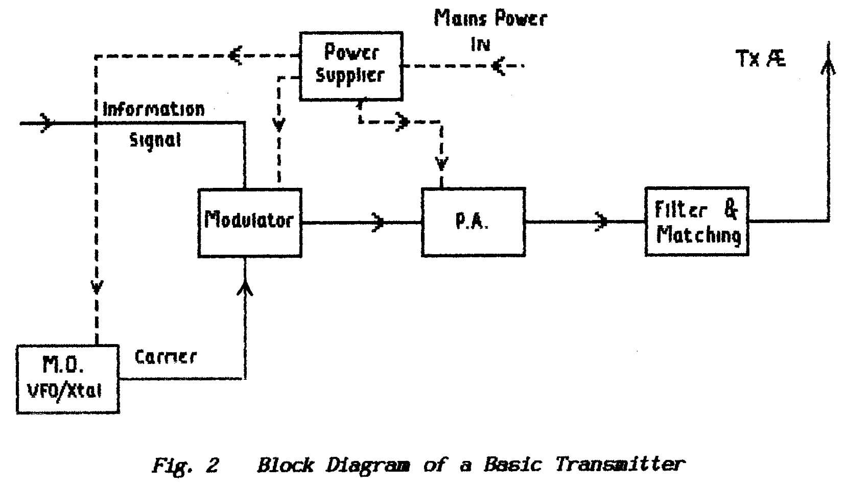
** Every transmitter has five main parts which are illustrated in Fig.2.
(i) The Master Oscillator or M.O.
>>>>>>>>>>>>>>>>>>>> PAGE 3 <<<<<<<<<<<<<<<<<<<<
(ii) A Modulator
(iii) The Power Amplifier or P.A.
(iv) Filter and Aerial-matching Units
(v) The Power Supplier
The first transmitters were called "spark transmitters" because they shocked a resonant LC circuit into trains of damped oscillations by discharging a series of sparks across a high-voltage spark gap; oscillations are dealt with in detail in Part 4: Electronic Oscillators. Sparks however are noisy things, electrically speaking, and the immense disturbance caused over a wide range of frequencies severely limited the number of transmitters able to operate simultaneously.
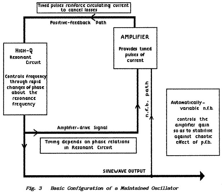
** The invention of the triode valve with its ability to amplify signals made it possible to maintain a resonant circuit in continuous oscillation. In an arrangement which utilises both positive-feedback and negative-feedback (see under 1.11 : Amplification in Lesson 5) the valve makes it possible to exercise tight control over the oscillatory process and so produce a stable single-frequency continuous sine-waveform; see Fig. 3. As a result the spark transmitter was outlawed and continuous-wave (c.w.) operation is the only accepted standard.
** The most important function of the Master Oscillator is to determine the desired frequency and, once set, to maintain that frequency constant. Stability of frequency is best achieved by utilising the very-rapid change of phase which occurs between voltage and current in a high-Q resonant circuit as it passes through resonance but, in practice, it is not all that easy to maintain the constant Q-value which is required. The greatest enemy is changes of temperature which cause:
>>>>>>>>>>>>>>>>>>>> PAGE 4 <<<<<<<<<<<<<<<<<<<<
(a) changes in the physical size of components which thus change their values of L and C
(b) changes in the properties of the materials used in constructing those components; this affects the values of L and C and also the leakage currents in semiconductor devices
(c) changes in the inter-electrode spacings of valves which change the circuit stray capacitances and so move the resonance frequency
(d) changes in the characteristics of valves and semiconductor devices which, by changing the circuit amplification, effectively changes the equivalent-circuit losses arid so affects the values of Q
** Variations in the power-supply voltage(s) also cause changes in device characteristics and, in semiconductors, changes in leakage currents and these too add their quota to the overall frequency drift.
>>>>>>>>>>>>>>>>>>>> PAGE 5 <<<<<<<<<<<<<<<<<<<<
** The Q-value of an LC circuit is dependent also on the effective load which is presented to it (the damping) and this can be changed either directly by variations in the load itself or through changes in stray couplings to local bodies.
** A M.O. therefore requires care in both its design and construction:
1. The resonant circuit is kept away from heat generating components
2. The resonant circuit is enclosed in a ventilated screening-box which ensures that stray couplings remain constant
3. The resonant circuit is coupled only loosely to the maintaining device (either valve or semiconductor) so that changes in its characteristics have minimum effect; this also results in the circuit being maintained at a minimum level of oscillation thus eliminating harmonic generation which also causes drift problems
4. The resonant circuit is coupled to the load by means of a buffer amplifier whose purpose is to provide isolation from load variations
5. All components associated with the resonant circuit are rigidly mounted to prevent changes of form being caused by mechanical shock
6. Power supplies for the maintaining device are carefully stabilised and are filtered and screened to prevent their providing an access path for intruding signals
7. Metering arrangements, which are necessary both for maintenance work and for the proper adjustment of the M.O., are also carefully filtered and screened.
** The majority of transmitters are required to work over a range of frequencies and so the M.O. is usually designed to be adjustable as discussed above ; this can be achieved by arranging for either the inductor or the capacitor (or both) to be adjustable. In most instances the capacitor is made variable because that is the easiest and cheapest method ; with reference to Section 1.13 however this method leads to variation in the circuit Q-values and so the oscillator stability varies across the tuning range if that range is excessive. In such transmitters the M.O. is referred to as the variable-frequency oscillator or the V.F.O.
** Transmitters which are required to operate on a single fixed frequency can achieve very high orders of stability and waveform-purity because the design can be optimised. Generally the LC resonant circuit is replaced by a mechanical resonator in the form of a thin slice of quartz crystal ; other forms of resonator are available today but the crystal probably provides the greatest accuracy and stability. These devices have the useful property of deforming mechanically when subjected to an electric voltage and, in reverse, of generating an electric voltage when they are mechanically deformed. Crystals can offer effective Q-values up to 30,000 but, with special mountings and careful circuit design, they can go as high as a half-million.
** When loosely-coupled to a maintaining circuit and lightly driven crystal-oscillators offer great immunity from frequency drift and this can be improved further by mounting the crystal in a temperature-controlled oven. Transmitters
>>>>>>>>>>>>>>>>>>>> PAGE 6 <<<<<<<<<<<<<<<<<<<<
which use a crystal in their M.O. are said to be crystal controlled and the M.O. is referred to as a Xtal. Osc.
** The range over which crystals can operate is limited. At the lowest limit around 2 kHz the crystal slice becomes a relatively massive bar and difficulty can be experienced in persuading it to oscillate. At the highest frequencies the slice becomes thin and fragile and is easily destroyed by over-driving. By cutting crystals to operate in so-called overtone modes (i.e. harmonic modes) it is possible to use them up to around 25-MHz. This range can be extended by using frequency-multiplying techniques and/or frequency-translating techniques which will be described fully under 2.2.4 and 2.2.5
** A continuous sinewave can also be generated by a technique known as frequency synthesis which does not require a resonant LC circuit or other device; however a crystal oscillator usually forms part of the arrangement because it provides the necessary frequency stability . In use as a transmitter drive these circuits are simply referred to as a V.F.O. They offer ease of adjustment, good frequency stability, good waveform and compactness but they do suffer from background noise. Also their frequency-adjustment is not continuous as with an LC arrangement ; the frequency changes in discrete intervals although the size of the interval is a matter of expense.
** The oscillator section of a transmitter plus any follow-on buffers, amplifiers and multipliers is often referred to as the . When a transmitter is used in conjunction with a separate receiver it is necessary to fit a drive-switch which, in the Receive position, shuts off the drive section. Without this facility radio- frequency (rf) signals leaking from the transmitter block the receiver to signals on the operating frequency. In Transceivers the transmitter and receiver are combined in a single unit ; the drive section is frequency-shifted and incorporated into the receiver when not transmitting and so the problem does not arise.
** The above Section on the Master-oscillator has described the Carrier-wave in terms of its frequency ; i.e. the number of complete cycles of oscillation that take place each second. Carrier signals are often referred to in terms of wavelength and the purpose here is to explore the relation and meaning of these two terms.
Light is an electromagnetic radiation which differs from radio waves only in that it has a much higher frequency. Early experiments which attempted to measure the speed at which light propagates produced the surprising result that the velocity of light appeared to be a constant ; i.e. the speed at which a light source moves or the speed of any observer receiving that light does not affect in any way the speed with which the light propagates from the Source to the Observer.
The meaning of this strange result was the basis of a theoretical discussion by one Albert Einstein who finished up with his oft-quoted Theory of Relativity which, fortunately, does not have any place in the R.A.E. This constant speed at which all electromagnetic radiation seemingly propagates is given the symbol e and has the value 3 x 10⁸ metres/second (or roughly 180,000 m.p.h.).
>>>>>>>>>>>>>>>>>>>> PAGE 7 <<<<<<<<<<<<<<<<<<<<
Electromagnetic waves at radio frequencies are generated by an aerial when it is excited by an alternating-current . The closely coupled electric and magnetic fields around the aerial constantly build to maximum values, fall to zero and then build again in the reverse direction and this repeating pattern propagates away from the aerial.
** Given that the carrier is being generated at a constant frequency (f) then successive peaks are generated at constant time intervals and this must mean that the peaks of the propagating field are separated by equal and constant distances. The distance between successive cycles - the distance traveled by an e-m wave during the time of one cycle - is known as the wavelength (λ).
** As the frequency is increased so the time interval for each cycle is decreased and so the wavelength must also decrease. This results in a simple relationship between frequency and wavelength linked by the constant velocity of propagation:
f x λ = e
Thus given either the frequency in cycles/second (Hertz) or the wavelength in metres the alternative form can be calculated by dividing the known value into 3 x 10⁸ .
** Questions involving this calculation are very likely to arise in the R.A.E. and the most likely cause of failure to earn easy marks is to forget that the basic units are cycles and metres. kHz should be expressed as f x 103, MHz as f x 106 and wavelengths expressed in metres.
END OF LESSON 1
* * * * * * * * * * * * * * * * * * *
QUESTIONS
1. Fig.1 shows the basic communication chain. What are the functions of the switches ?
2. The propagation path was said to be the least reliable link in the communication chain. What particular facility must it offer that is most likely to cause a failure in communication ?
3. Detail the parts of a transmitter and state briefly their function.
4. What is the difference between a VFO and a Xtal.Osc. 7 ?
5. On what equipment would you expect to find a "Drive" switch and for what purpose would you use it ?
6. Confronted with a working transmitter how would you determine whether it
was fitted with a standard VFO or
a Synthesiser without going inside ?
7. What is the frequency of a carrier operating on 20.2 metres ?
What is the wavelength when the carrier frequency is
(a) 805 kHz & (b) 15.15 MHz 7
>>>>>>>>>>>>>>>>>>>> PAGE 7(again) <<<<<<<<<<<<<<<<<<<<
** The process of loading a carrier wave with information is called modulation and the circuit arrangement which carries out the task is called a modulator. The purpose is to vary one of the characteristics (one of the parameters) of the carrier-wave in accordance with the form of the information signal.
** The simplest modulation system switches the carrier on and off in a series of long and short bursts to form the internationally-accepted Morse Code. The message is spelled out one character at a time ; although laborious the code can be both sent and read by experienced operators as easily as they read the human voice. Because of the distinctive rhythms of the characters a message can be read against a background of noise that completely obliterates all other systems.
An early version of this type of modulation was known as interrupted continuous-wave (I.C.W.) in which the carrier was regularly interrupted by a buzzer or a tonewheel mechanism. If the interruptions occurred at audio frequency then the presence of the carrier appeared as an audible tone at the output of a simple receiver. A cw carrier produces only dc at the receiver output and additional components are necessary to make the incoming signal audible. (See under 2.6 Receivers.)
CW-working is often referred to as carrier-wave working but the initials stand for continuous-wave as distinct from the discontinuous wave-trains of the early spark transmitters. To the pedant the unmodulated wave cannot be a "carrier" but it can be argued that morse is indeed a form of modulation because it does produce sidebands (described below). In practice confusion does not result and the exact meaning of the nomenclature is not important.
** There are four basic ways in which a carrier can be modulated:
(a) by variation of the carrier amplitude - amplitude modulation(A.M.)
(b) by variation of the carrier frequency - frequency modulation(F.M.)
(c) by variation of the carrier phase - phase modulation (Ph.M,)
(d) by pulsing the carrier - pulse modulation(P.M.)
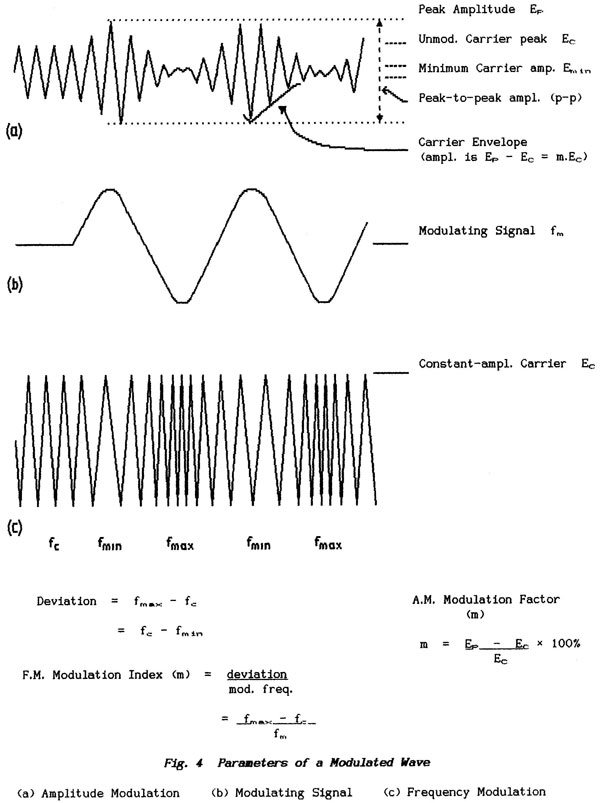
(a) Amplitude Modulation is a system in which the amplitude of a carrier-signal is varied according to the form of a modulating signal; see Fig.4. Maximum possible depth of modulation (100% modulation) occurs when the carrier amplitude varies from twice the unmodulated value down to zero; modulation is normally limited to around 80% to avoid distortions which arise from the limitations of circuitry and not from the modulation process itself.
** Where the modulating signal consists of a single frequency (or tone) the resulting modulated carrier is termed a modulated continuous-wave (M.C.W.) and this can be used for Morse-code transmissions either by keying the carrier or by keying the modulation. The advantage of keying the modulation is that the carrier remains at a constant amplitude during the "spaces" and serves to quell the noise that otherwise appears at the receiver output but the method is seldom used today except occasionally with F.M. ICW operation mentioned above is a special instance of M.C.W. used with A.M.
** To vary the amplitude of a carrier-wave it is necessary to cause a small amount of distortion from cycle to cycle and so a modulated carrier cannot be
>>>>>>>>>>>>>>>>>>>> PAGE 8 <<<<<<<<<<<<<<<<<<<<
>>>>>>>>>>>>>>>>>>>>
PAGE 9
<<<<<<<<<<<<<<<<<<<<
regarded as a pure single-frequency carrier. In fact, for every frequency in the modulating waveform, two extra near-carrier frequencies are produced one on each side of the carrier proper ; if fc is the carrier frequency and fm, is the modulating frequency then the additional two frequencies produced by A.M. are fc + fm and fc - fm.
** These two extra frequencies are properly referred to as side frequencies ; a group of side frequencies either above the carrier frequency or below it are called a sideband and they are designated either as the upper sideband or the lower sideband. In common parlance however they are usually referred to collectively as the sideband frequencies or simply as the "sidebands"
** In a 100% modulated A.M. carrier one-third of the total emitted power resides in the sidebands and each sideband contains all the modulated information . It follows that the full double-sideband amplitude-modulated signal wastes 5/6 of its total power and that it occupies a band of frequencies which is twice that strictly necessary.
** Modulator circuit techniques make it possible to remove the carrier and leave only the two sidebands; in such a suppressed-carrier system the total emitted power is divided equally between the sidebands but still 50% of the power is wasted in duplication and the bandwidth is still twice that necessary.
** A suitable filter can be placed after the Modulator to remove either the upper or the lower sideband and the result is known as a single-sideband (ssb) emission. In such a signal all the emitted power is utilised to carry information and the bandwidth is half that of the parent A.M. signal.
** In Radio-telephony (R/T , voice or 'phone) ssb is now the only form of A.M. which is tolerated . (Note that, on the Amateur Bands, it is accepted that the lower sideband is used for 160, 80 and 40 metres (1,8, 3.5 & 7.0 MHz) and the upper sideband for all other transmissions.
** Sidebands are produced only when information is modulated on to a carrier; when the modulating signal is zero then only the carrier signal is present. In ssb operation that carrier is removed and so it is characteristic of ssb that the transmitter output remains at zero until the Operator speaks into the microphone. Thus a power meter or an s.w.r. meter, which usually are connected between transmitter and aerial system, remains quiescent until the Operator begins to speak.
** (b) Frequency Modulation is a system in which the carrier amplitude is maintained at a constant value but the frequency is varied according to the form of a modulating signal. There is a clear limitation to this system in that the carrier frequency cannot be allowed to approach zero ; in fact it cannot be taken very far at all expressed as a percentage of the normal (unmodulated) frequency. Thus F.M. tends to be used only with high carrier frequencies.
** The depth of modulation is expressed as a modulation index which indicates the relation between the frequency of the modulating signal (i.e. the rate at which the carrier frequency is being shifted) and the extent of the frequency shift at the peaks of the modulating waveform. The range over which the carrier frequency is swung is known as the frequency deviation ; see Fig. 4.
** Although the amplitude of a F.M. carrier is kept constant it is still true that distortion occurs from cycle to cycle as the frequency is continuously varied and so this modulation system too produces sidebands. Any modulation system must
>>>>>>>>>>>>>>>>>>>> PAGE 10 <<<<<<<<<<<<<<<<<<<<
produce sidebands because that is where the information lies. The modulated carrier is no longer a pure single-frequency waveform ; for every frequency in the modulating signal pairs of sideband frequencies appear either side of the carrier. When the modulation-index is less than 0.5 the F.M. signal is similar to an A.M. signal but, as the deviation is increased, so more sideband frequencies appear spaced at intervals which are equal to the modulation frequency fm . The bandwidth of the modulated signal is approximately the deviation plus fm.
** With F.M. it is not possible to remove the carrier and so this system is not as efficient in its use of power as a ssb system ; where large values of deviation are used the F.M. signal spreads over a large portion of the frequency spectrum which is another reason why its use is generally confined to the higher carrier frequencies (see under 1.14: Relative Bandwidth).
** Practical modulators are not as co-operative as one might wish and they invariably produce A.M. as well as F.M. This usually is dealt with by using a limiter stage after the Modulator which removes the A.M. (With A.M. systems a poorly-designed modulator is equally likely to produce F.M. as well as A.M.).
** Despite their wide bandwidth and inefficient use of power F.M. systems play an important part in communications because of their relative immunity to noise. Most forms of interference cause changes of amplitude; because such changes are not significant when using F.M. the receiver can pass an incoming signal through a limiter stage thus obtaining a carrier with a constant (noise-free) amplitude with only F.M. remaining.
** There are two minor drawbacks to F.M. working which arise when the received signal level becomes too small:
(a) noise takes over very abruptly as the limiter fails
(b) an unwanted signal on the same or close-by frequency suppresses the wanted
modulation and substitutes its own in a process known as Capture
Effect
(c) Phase Modulation is a system in which the phase of the carrier is changed (its timing is changed) according to the form of a modulating signal ; the frequency is held constant but the carrier is shifted in Time. However it can be argued that the difference between phase modulation arid frequency modulation is more a matter of mathematical definition and, in practice, the greatest difference lies in the techniques used to achieve the modulation. A detailed knowledge of Ph.M. is not required f or the R.A.E.
Suffice it to say that, to shift a carrier-wave in Time, it is necessary momentarily to either stretch the waveform or to compress it and this involves a momentary change of frequency ; for a continuously-varying modulation signal clearly the frequency change is continuous also. The argument operates in reverse in that, to change the frequency of a carrier-wave, its timing (or phase) must be changed. It is not proposed to go further than this simplified approach.
(d) Pulse Modulation is a system in which the carrier is pulsed ; i.e. it is generated in short bursts very similar to an I.C.W. system except that the pulses occur at a rate well above the audio range.
>>>>>>>>>>>>>>>>>>>> PAGE 11 <<<<<<<<<<<<<<<<<<<<
>>>>>>>>>>>>>>>>>>>> PAGE 12 <<<<<<<<<<<<<<<<<<<<
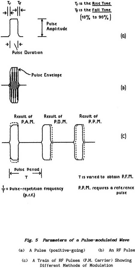
Fig. 5(a)shows a pulse as it would be generated in an electronic circuit (note that the term "impulse" is now obsolete) and diagram (b) shows the rf pulse or rf burst which results when a pulse is used to modulate a carrier. Diagram (c) shows a train of such rf-pulses in the form of a pulse-modulated carrier.
A pulse-modulated carrier can be used in a variety of ways and for a variety of purposes
(a) Pulse-amplitude Modulation (P.A.M.) is a system in which the pulse-amplitude is varied according to the form of a modulating signal.
(b) Pulse-duration Modulation (P.D.M.) is a system in which the pulse duration (its length in Time) is varied according to the form of a modulating signal.
(c) Pulse-position Modulation P.P.M.) is a system in which the positions (in time) of the pulses are varied according to the form of a modulating signal.
(d) Pulse-frequency Modulation (P.F.M.) is a system in which the pulse repetition rate (p.r.f.) is varied according to the form of a modulating signal.
(e) Pulse-code Modulation (P.C.M.) refers in general to any system in which the pulses are modulated according to a predetermined pulse-code.
Pulse modulation is particularly useful in systems which seek to send several different information signals simultaneously over a single channel ; such systems are known as multiplex systems. In a time-division multiplex equipment the channel is shared between different information signals on a time-rota basis and, using P.C.M., this can be done by modulating each signal on to selected pulses in the train. For example, to carry three signals, the first information signal would be modulated on to pulses 1, 4, 7, 10 etc.; the second information signal would be modulated on to pulses 2, 5, 8, 11 etc.; the third information signal would be modulated on to pulses 3, 6, 9, 12 etc. The pulses are sorted at the receiving point by use of a gate circuit which directs pulses to the appropriate destination channels.
** Pulse-modulation techniques are permitted by the Amateur Licence with certain restrictions that are laid down in the Licence document itself as well as in the Licence Regulations. The matter is not examined for the R.A.E.
END OF LESSON 2
* * * * * * * * * * * * * * *
QUESTIONS
1. What is meant by the term "Modulation" ?
2. Why does a modulated carrier-wave no longer behave as though it were a single-frequency wave ?
3. A carrier on 1.8 MHz is modulated simultaneously by signals at 100 Hz (hum), 1 kHz and its third-harmonic at 3 kHz. What are the various frequencies that emerge from the modulator circuit ?
4. State the major advantage and the major disadvantage of an F.M. channel
5. When a transmitter is switched on it fails to produce an output signal. What is the probable reason for this and how would you check the diagnosis ?
>>>>>>>>>>>>>>>>>>>> PAGE 13 <<<<<<<<<<<<<<<<<<<<
** It is difficult to build high-frequency oscillators which are stable in frequency and so, in general, master oscillators are designed to operate at low frequencies. To achieve good stability and accuracy in setting they need also to be designed so that they cover only a small band of frequencies. The output from a M.O. is then converted to the frequency range at which the output is required
** Crystals have limited ranges of operation and so frequency-conversion is necessary also if crystal oscillators are to be used above 25 MHz.
** The frequency-conversion process can be carried out in two different ways namely frequency-multiplication or frequency-translation.
** Frequency-multiplication involves deliberately distorting the waveform of the M.O. output so as to generate harmonic frequencies ; the required harmonic is then selected by a suitably-tuned resonant circuit and then amplified in a tuned rf- amplifier. Such a multiplier stage is driven by the constant-frequency signal of the M.O. and so, despite the waveform distortion, the frequency stability is maintained. Note that the waveform within the M.O. must not be distorted else frequency drifting must occur (effective reduction of Q).
** One limitation of this technique is obvious in that the required final frequency has to be a harmonic of the M.O. frequency but this is not a problem when the M.O. is variable and so the necessary fundamental frequency is obtainable.
** A second limitation is that the generated harmonics have to be kept within the frequency—multiplying stage and not allowed either to appear in the final output signal or to radiate from the equipment.
A ** A third limitation is that the frequency—multiplying action operates also on any side frequencies that may be present which means that the modulating frequencies are multiplied also ; the actual effect depends on the modulating system in use :(a) Effect of Multiplication on A.M. Signals
Consider a carrier of frequency 1 MHz which is amplitude-modulated at I kHz: the side frequencies therefore are 999 kHz and 1,001 kHz . When such a modulated carrier is subjected to a frequency multiplication of 10 the result is a carrier at 10 MHz flanked by side frequencies at 9.99 MHz and 10.01 MHz . This represents a modulating frequency of 10 kHz and demonstrates that the modulation also has been multiplied by 10.
** With A.M. therefore it is necessary to carry out all multiplying operations before applying the modulation.
The same argument applies to any frequency-drift of the M.O. ; a change of 1% from 1 MHz to 1.01 MHz (admittedly a poor oscillator) would appear at the multiplier-output as a change from 10-MHz to 10-1 MHz. This still represents a drift of 1% but the increased change of frequency, as measured in cycles-per-second might well take the carrier outside the bandwidth of the 10-MHz circuits.
>>>>>>>>>>>>>>>>>>>> PAGE 14 <<<<<<<<<<<<<<<<<<<<
(b) Effect of Multiplication on F.M. Signals
Consider a carrier of frequency 1 MHz which is frequency-modulated by a signal at fm hertz with a deviation of I kHz (i.e. the carrier swings from 999 kHz to 1.001 MHz). Frequency multiplication by a factor of 10 will again result in a carrier at 10 MHz but with a deviation from 9.99 MHz to 10.01 MHz. The rate at which the carrier is swung between 9.99 MHz and 10.01 MHz will not be affected and so the modulating frequency remains unchanged.
** With F.M .therefore modulation can be effected either before or after frequency-multiplying operations are carried out. However, the modulation-index is increased because the deviation has been increased while the modulating- frequency remains unchanged. This implies that more side-frequencies have been generated on either side of the carrier and these are spaced at intervals equal to the modulation frequency fm.
** Although frequency-multiplication does not of itself increase the relative-bandwidth(bandwidth relative to the centre frequency) the change of modulation-index increases the spread of the signal. When designing or aligning a F.M. transmitter the deviation must be set at the output of the modulator stage so as to achieve the desired modulation-index at the output of the multipliers.
The problem of frequency-drift in the M.0. remains the same as in A.M.
To translate means to move to another place or, in this instance, to move a signal "sideways" through the frequency spectrum to another position. Thus a carrier on 1 MHz might be translated to 5.4 MHz which is an operation that cannot be carried out with the frequency-multiplication technique. Frequency translation is also the only means of shifting a signal down the spectrum to a lower frequency.<
** Frequency translation is achieved by mixing the basic carrier with another sinusoidal waveform. As shown under 2.2.3 and in Fig. 6 when two sinewaves are mixed then, either in a linear circuit or in a nonlinear circuit, two extra sinewaves are generated with frequencies that are the sum and difference of the two parent frequencies.
Thus, with reference to the 1-MHz carrier mentioned above, to translate it to 5.4 MHz it must be mixed with either a 4.4-MHz signal or with a 6.4-MHz signal.
The carrier might have been derived from a VFO which ranged from 0.5 MHz to 0.8 MHz; the signals available at the output of the frequency-translater would be:
with 4.4-MHz 3.9 to 3.6 MHz (f1 — f2)
4.9 to 5.2 MHz (f1 + f2)with 6.4-MHz 5.9 to 5.6 MHz (f1 — f2)
6.9 to 7.2 MHz (f1 + f2)
Such a combination of VFO, two oscillators and a frequency-mixer could, when equipped with suitable filters and switching, cover four ranges of frequencies
3.6 to 3.9 MHz
5.6 to 5.9 MHz
4.9 to 5.2 MHz
6.9 to 7.2 MHz
>>>>>>>>>>>>>>>>>>>> PAGE 15 <<<<<<<<<<<<<<<<<<<<
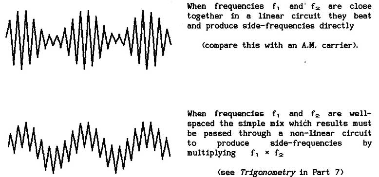
Fig. 6 Result of Mixing Two Sinewaves
The secondary signal is not required to vary and so it can be derived from a fixed-frequency oscillator of optimised design which is crystal controlled. Crystal oscillators are capable of frequency stabilities of 1 part in 10,000 (1 cycle at 10-kHz) without special precautions ; with specially-designed crystals mounted in temperature-controlled ovens stabilities up to 1 part in 106 or even greater can be achieved and this has a beneficial effect on the overall performance of the M.0. system.
The 1-MHz oscillator mooted above was given a poor stability of 1% (1 part in 100); when mixed with a secondary-oscillator output with a stability of 1 in 104 the stability of the frequency-translated output can be calculated as follows:
Carrier at 1 MHz mixed with waveform at 4.4 MHz results in a translated carrier at 5.4 MHz. When the carrier drifts to 1.01 MHz the translated carrier drifts to 5.41 MHz. Maximum drift of the secondary oscillator is from 4.4 MHz to 4.4004 MHz and this will move the translated carrier further out to 5.41044 MHz if both oscillators drift in the same direction.
This represents an overall drift (maximum drift) of approximately 1,044 parts in 540,000 which is approximately 1 : 540 or 0.2 % Thus, in terms of the translated output, there has been a 5-fold improvement in the frequency-stability. Note too that, where the carrier is derived from a VFO, that Master Oscillator works always over the same range ; were a simple oscillator used with switching to cover the two ranges 0.5 to 0.8 MHz and 10.5 to 10.8 MHz it would be necessary to cope with relative ranges of 50% for the first mode and 3% for the second.
>>>>>>>>>>>>>>>>>>>> PAGE 16 <<<<<<<<<<<<<<<<<<<<
The effect of frequency-translation on different modulation systems is important too:
(i) Amplitude Modulation
** Consider a carrier at 1 MHz modulated at 1 kHz and which therefore has side-frequencies at 999 kHz and 1,001 kHz. When mixed with the 4.4-MHz secondary signal the carrier is translated to 5.4 MHz and the side-frequencies to 5.399 MHz and 5.401 MHz . This still represents a modulating frequency at 1-kHz ud so translation can be used either before or after modulating a carrier; one instance of such is found in the superheterodyne receiver described later in the Course.
** The relative bandwidth is decreased when a carrier is translated to a higher frequency and correspondingly increased when a carrier is translated to a lower frequency.
(ii) Frequency Modulation
** Consider a carrier at 1 MHz modulated by a signal at fm with a deviation of 1-kHz. When mixed with a secondary signal at 4.4 MHz the carrier is again translated to 5.4 MHz and the frequency-swing (twice the deviation) becomes 5.399 to 5.40 1 MHz . The rate at which the carrier-frequency is swung remains unchanged and so the modulating frequency remains unchanged. Thus frequency-translation too can be used either before or after modulating a carrier.
However the deviation has remained at ±1 kHz and so the modulation-index has not been changed ; in turn this means that the range of side-frequencies has not been changed with the increase of carrier frequency. Thus the relative bandwidth (see under 1.14.1 on p.64 of Fundamentals—1) has been reduced as a percentage of the carrier frequency.
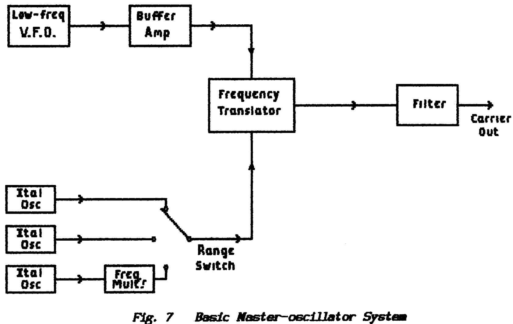
** From the above it is to be concluded that the best M.0. systems are based on the general arrangement shown in Fig. 7and require:
>>>>>>>>>>>>>>>>>>>>
PAGE 17
<<<<<<<<<<<<<<<<<<<<
(i) a low-frequency VFO which is capable of covering the greatest required range of frequency as measured in cycles-per-second.
(ii) a frequency-translating system which uses well-designed fixed-frequency oscillators (preferably crystal-controlled oscillators) with best-possible frequency stability to convert the output of the VFO to the required ranges. By providing a choice of such oscillators, with frequency-multipliers as necessary, the M.O. can be switched to cover different ranges of operation while preserving the frequency stability of the fixed-range low-frequency VFO.
Transmitters which are intended for operation on a fixed frequency may use frequency-multipliers to arrive at the final output frequency provided that the oscillator is sufficiently stable for the final output-signal drift to be within tolerance. In such transmitters however care is necessary to ensure that the many harmonics which are generated neither appear in the final output signal nor radiate directly from the transmitter casing. Thus an important part of a transmitter drive-section is adequate filtering, screening and buffering.
END OF LESSON 3
* * * * * * * * * * * *
QUESTIONS
1. In the Master-oscillator section of a transmitter why is it desirable to indulge in frequency-changing ?
2. What is the difference between frequency-multiplication and frequency-translation ? Each technique has its merits ; what are they ?
3. Why is it not possible to amplitude-modulate before frequency-multiplication is undertaken ?
4. Describe the basic technique used in frequency-translation.
>>>>>>>>>>>>>>>>>>>> PAGE 18 <<<<<<<<<<<<<<<<<<<<
Although frequency synthesisers produce more background noise then standard oscillators they are useful in that they are compact and can produce a variable frequency with a stability close to that of a crystal oscillator . They have a minor disadvantage in that the frequency can be adjusted only in discrete steps but the size of those steps is a matter of cost rather than technical difficulty.
** The output signal from a synthesiser is locked in frequency to that of a reference signal which may be either
(a) an internal crystal-controlled oscillator
(b) an externally-supplied signal.
For many uses, including amateur radio, the stability of a well-designed crystal oscillator without a crystal oven is sufficient and so a synthesiser which uses an internal crystal-oscillator as a reference can be used as a VFO. Provision for alternative use of an external reference allows the VFO to be locked to such things as a local frequency-standard or to the mains frequency; this last can be useful in avoiding the adverse effects of mains-induced hum.
The inference therefore is that frequency-synthesisers translate either upward or downward from the frequency standard but they differ from the translating techniques already described in that they retain the stability of the standard. This is achieved by use of a Phase-locked Loop (PLL). Despite its intimidating name this device is simply an implementation of the basic servo-system which was described in Lesson-5 of Fundamentals-1under 1.11: Amplification.
The two diagrams given in Fig. 13of that Lesson are based on signals that vary continuously and which are described as an analogue system. The PLL makes use of digital techniques in which signals are handled as a series of numbers.
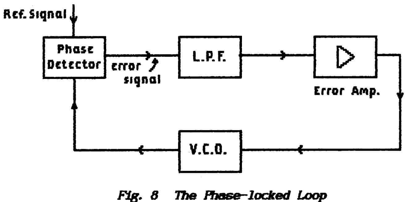
** The basic PLL is shown in Fig. 8 and it consists of four parts:
(a) a voltage-controlled oscillator (VCO) usually tuned by a varactor diode or a varicap
(b) a phase-detector or phase-comparator
(c) a low-pass filter (LPF)
(d) an error-signal amplifier
>>>>>>>>>>>>>>>>>>>> PAGE 19 <<<<<<<<<<<<<<<<<<<<
** The phase-detector compares the outputs from the VCO and from the reference source; it produces an error signal which is proportional in magnitude and in polarity to the manner in which the two signals differ in phase. Ideally, with the system in a stable condition, this error-signal is either zero or a small-value dc and the purpose of the LPF which follows the detector is to ensure that all other "noise" signals are excluded.
** The error-signal is applied to the voltage-controlled oscillator to adjust its frequency in such a way that any phase-error is reduced. With the system properly adjusted the frequency of the VFO is locked to that of the reference source ; any residual phase-error is indicated by the magnitude of the error-signal.
Note that, if the two frequencies are not identical, the two signals must constantly change their relative phase and the error-signal becomes a small- amplitude sinewave. In some applications of the PLL this sinusoidal signal is the required output signal but a simple use for the basic PLL as just described is that the output from the VCO is a "cleaned-up" version of a noisy reference signal.
As described so far the basic PLL does not differ from the system illustrated by Fig. 13 of Fundamentals-I; it could be purely analogue in its operation. In use as a frequency-synthesiser it requires also another type of unit known as a frequency-divider. As already described the frequency of a signal can be multiplied by distorting the waveform and selecting from the harmonics thus generated ; to divide the frequency of a signal so as to produce a sub-harmonc it is necessary to use digital techniques.
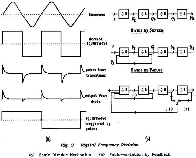
To compare phases or to count cycles it is necessary to identify accurately the same part of a waveform in each and every cycle. The best way with a sinewave, and usually with most other waveforms, is to use the zero-crossings; i.e. the moment that the signal passes through zero. To do this the sinewave is first greatly amplified in a limiting-amplifier so that it is turned into a square wave; in this way the zero-crossings become almost instantaneous as the signal level changes abruptly between two fixed levels. This is illustrated in Fig. 9.
The squarewave is then passed through a differentiating circuit (to be described later) which produces short pulses that are derived from the zero-crossing "edges" of the squarewave; positive-going transitions produce positive-going pulses and the negative-going transitions produce negative-going pulses. Either the positive-going pulses or the negative-going pulses are removed by use of a one-way device (a diode) so that the final output is a string of unidirectional pulses, one for each cycle of the input waveform . Clearly these pulses have a repetition rate which is equal to the input frequency and they are rigidly locked to the input (the driving) waveform.
A squarewave generator (as distinct from the limiting amplifier described above) is a circuit arrangement which changes its output between two fixed levels and it can be arranged that it executes these changes each time it receives an input pulse. When a string of pulses, such as that derived above, is applied to a squarewave generator the output-waveform that it produces is a squarewave at half the frequency of that applied to the differentiating circuit.
>>>>>>>>>>>>>>>>>>>> PAGE 20 <<<<<<<<<<<<<<<<<<<<
A comparison of the input and output frequencies of the system thus leads to the conclusion that the circuit has divided the input frequency by a factor of 2 and so the system is referred to as a binary counter or a binary divider.
** By cascading several of these binary stages it is possible to produce circuits which divide by 2, 4, 8, 16, 32, etc.; the output from each successive stage represents division by factors of 2, 22, 23, 24, etc. Compare this "scale-of-two" counting system with our more normal "decimal" or scale-of-ten system in which each successive counter registers a power of 10; writing 137 means add together (102) + (3 x 10) + ( 7 x 1) .
In modern electronics it is not necessary to design squarewave generators, pulse-forming circuits and all the necessary ancillaries to make frequency dividers; they come ready made in the form of "chips".
The type of binary counter described above is much used in computers. When a string of pulses is entered the first pulse affects only the first binary stage; the second pulse causes the first stage to reset to its original condition and, at the same time, to "hand-on" a pulse to the second stage; the fourth input pulse causes the second stage to reset and hand-on a pulse to the third stage; the eighth pulse causes the third stage to reset and hand-on a pulse to the fourth stage and so on. Thus, if the string of dividers is examined to determine the
>>>>>>>>>>>>>>>>>>>> PAGE 21 <<<<<<<<<<<<<<<<<<<<
state of each stage, it is possible to deduce the number of pulses that were applied to the input.
A string of binary counters used in this way is known as a shift-register because successive stimulation at the input causes the change-of-state to shift along the string from stage to stage. In computing circles it is usual to refer to the arrangement simply as a Register, meaning a device which will hold a (binary) number; however, it can be much easier to understand a computer if it is remembered that a register has the function of shifting numbers and that they can be made to shift in either direction (distinguished as "counting-up" and "counting- down"). This is a most important concept in getting computers to calculate.
** The final trick with a binary string is to turn it into a decimal counter by employing feedback techniques; pulses are extracted from appropriate stages and fed-back to earlier stages so as to cause "false" triggering. For example, if the output pulse from a divide-by-four is fed back to its input, then every third pulse will generate a feedback-pulse which takes the place of a would-be fourth input pulse; the one-time divide-by-four has thus become a divide-by-three. Other examples are shown in Fig. 9. Note that feedback reduces the count.
Again with modern electronics the whole process is contained within a single chip in which the division-ratio can be set by making appropriate connections externally between specified pins. A single chip may contain more than one counter-chain. Such a device is no longer a binary-counter and it is usual to refer to it as a frequency-counter or perhaps more usually as a frequency divider.
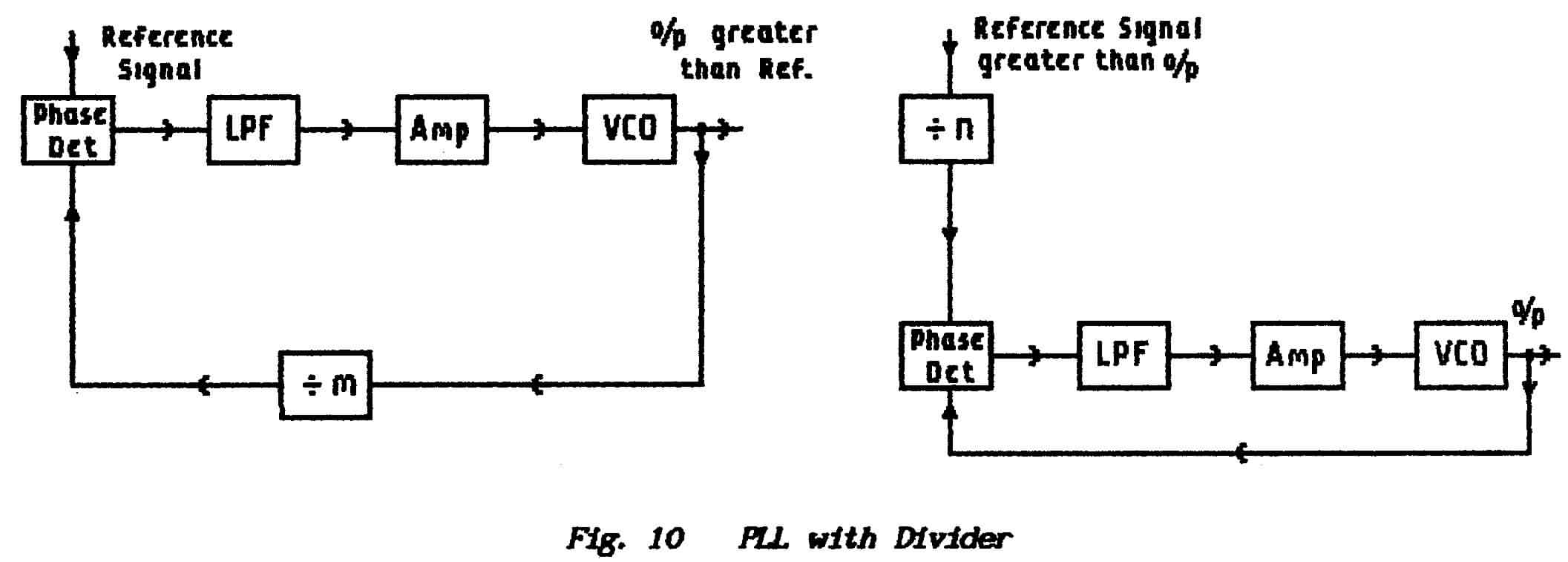
** To make a frequency-synthesiser a PLL-oscillator is combined with a frequency-divider and there are two possible positions for it as shown in Fig. 10.
** With the divider between the VCO and the phase-detector the synthesiser can operate with the frequency of the VCO greater than the frequency of the reference signal; with the divider between the reference and the phase-detector the synthesiser operates with the frequency of the VCO less than that of the reference.
A combination of both techniques makes the device extremely flexible. By dividing both signals to a common factor it becomes possible to produce almost any frequency from the VCO. To produce a frequency-stable but variable oscillator
>>>>>>>>>>>>>>>>>>>> PAGE 22 <<<<<<<<<<<<<<<<<<<<
unit all that is necessary is to provide a means of switching the feedback connections which control the operation of the two dividers.
However, the operation of the phase-comparator requires that the dividers produce a common factor of the two frequencies; this means that the output from a synthesiser can be adjusted only in discrete steps. The size of those steps depends on the number of decimal places available in the division-ratio and so determines the cost of the arrangement. See Fig.11.
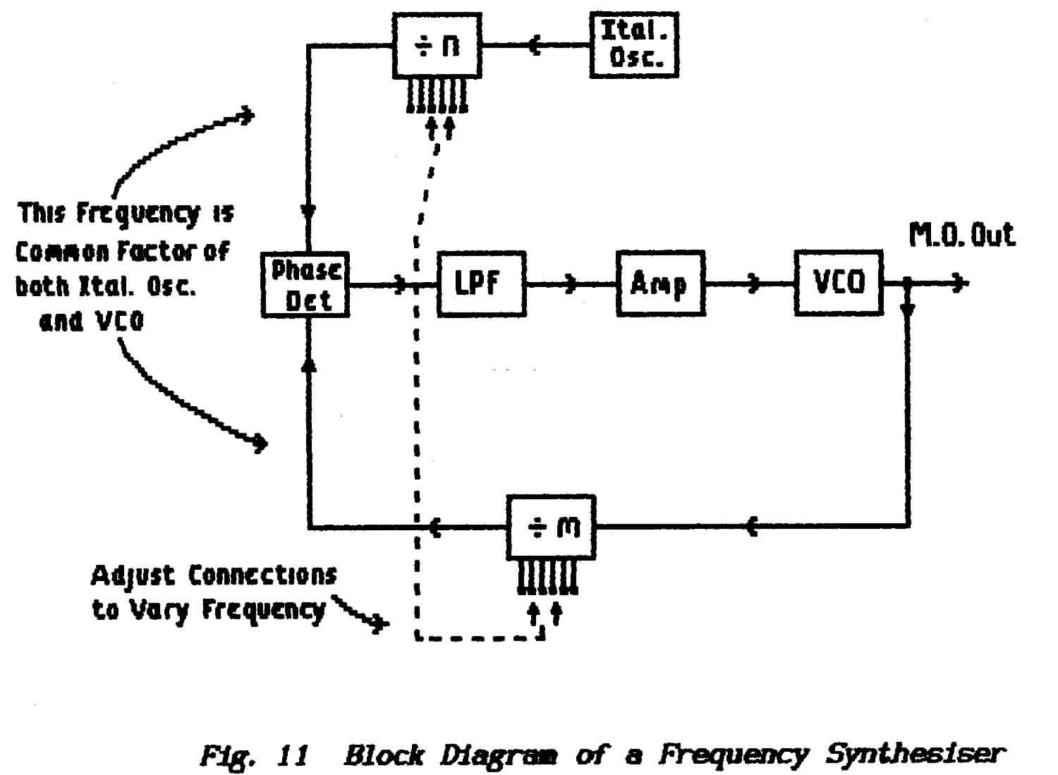
(You should be familiar with this diagram for the R.A.E.)
>>>>>>>>>>>>>>>>>>>> PAGE 23 <<<<<<<<<<<<<<<<<<<<
END OF LESSON 4
* * * * * * * * * * * *
QUESTIONS
1. Why does a frequency-synthesiser use a reference signal ?
2. Drew in block form a basic Phase-locked Loop arrangement and describe its action. (You might well receive a question of this nature in the R.A.E.)
3. Given that the error-signal in a PLL is a dc why can you be sure that the two oscillators are locked to the same frequency ?
4. Drew a chain of binary counters with feedback connections to give a division ratio of (a) 17 (b) 33 . (Not required for R.A.E.)
5. Draw in block form a frequency synthesiser and describe its action.
(Questions do appear on this subject in the R.A.E. although you would
not be required to draw the arrangement - multiple choice is used,)
6. At the bottom of Page-18 in this Lesson there is reference to a Varicap. What is this device ?
7. An LC oscillator is required to work over the range 1.0 to 1.7 MHz . A tuning capacitor is available which can be varied from 100 pF to 300 pF. Calculate a suitable value for the inductance required.
>>>>>>>>>>>>>>>>>>>> PAGE 23(again) <<<<<<<<<<<<<<<<<<<<
The Modulator is that part of a transmitter which accepts both a carrier-signal and a modulating-signal and modulates the one with the other. It is a circuit arrangement in which one of the carrier parameters is altered according to the waveform of the modulation.
(a) Amplitude Modu1ation
The simplest form of amplitude modulator consists of a radio-frequency amplifier in which the output power depends on the value of the modulating-signal waveform. This is achieved either by using the modulating signal to vary the auxiliary power supplier or by varying the characteristics of the amplifying device (either a valve or a transistor).
A fully-modulated A.M. carrier has one-third of its total power in the sidebands ; this is another way of saying that modulating a carrier increases its total power by 50% and this additional power represents the information which has been added to the carrier. This extra power is drawn from the auxiliary power-supplier under the control of the modulating signal.
** A simple way to do this is to amplify the modulating signal. to high power and then to connect this in series with the auxiliary power-supplier in an arrangement similar to that shown inFig.12(a). This is called anode modulation in valve
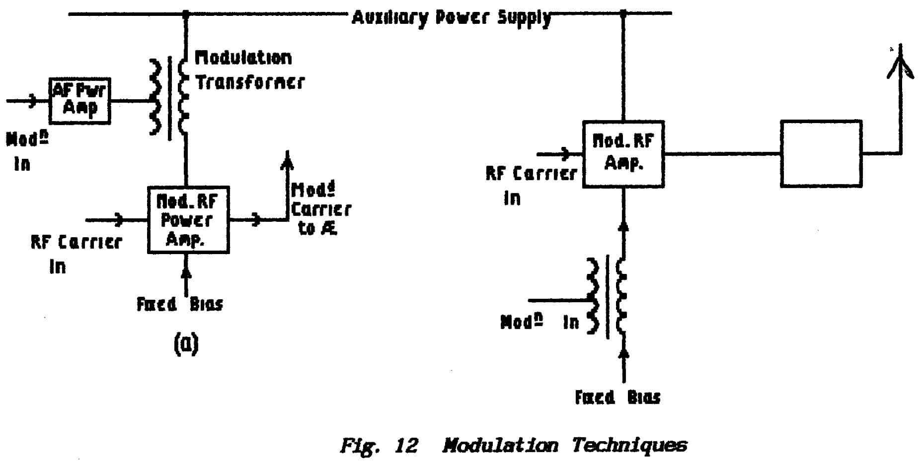
(a) Power Modulation in Class-C Rf-amplifier
(b) Low-power Modulation by Variation of the Bias circuits or collector modulation in transistor circuits. The diagram shows the power-signal coupled into the auxiliary-power feed by means of a transformer. There are a few points to note:
(i) The modulation transformer must be able to handle the power of the modulating signal and also be able to carry the direct current drawn by the rf-amplifier.
>>>>>>>>>>>>>>>>>>>> PAGE 24 <<<<<<<<<<<<<<<<<<<<
(ii) The modulation transformer must be insulated well enough to withstand the high voltages encountered in a valve rf-amplifier.
(iii) The audio amplifier which is supplying the modulating signal must be able to supply audio power (i.e. current as well as voltage) to at least 50% of the carrier power.
** For high-power transmitters (and especially so in those that use valves) anode modulation requires the use of expensive high-voltage units but it allows the rf-amplifier to be operated in the most efficient mode known as Class-C operation(see Part 3 of this Course). Anode modulation of a Class-C valve amplifier can result in very-low distortion levels and provides the greatest power output for a given size of valve . The circuit is also much easier to adjust than the alternative methods of modulation. The problems that arise from high-power working however are not a consideration for relatively low-power amateur transmitters and so this arrangement is often used.
** The type of modulator circuit shown in diagram (b) uses the modulating signal to vary the stage-gain of the rf-amplifier thus causing the output power to vary according to the modulation waveform. Usually this is done at low power-levels and the resulting A.M. signal must then be amplified to the final output power by means of one or more non-distorting rf-amplifiers. For distortion not to occur the output power must always be proportional to the value of the input waveform: plotted as a graph of output versus input the result is a straight line and so this type of amplifier is referred to as a linear amplifier or more simply as a "linear".
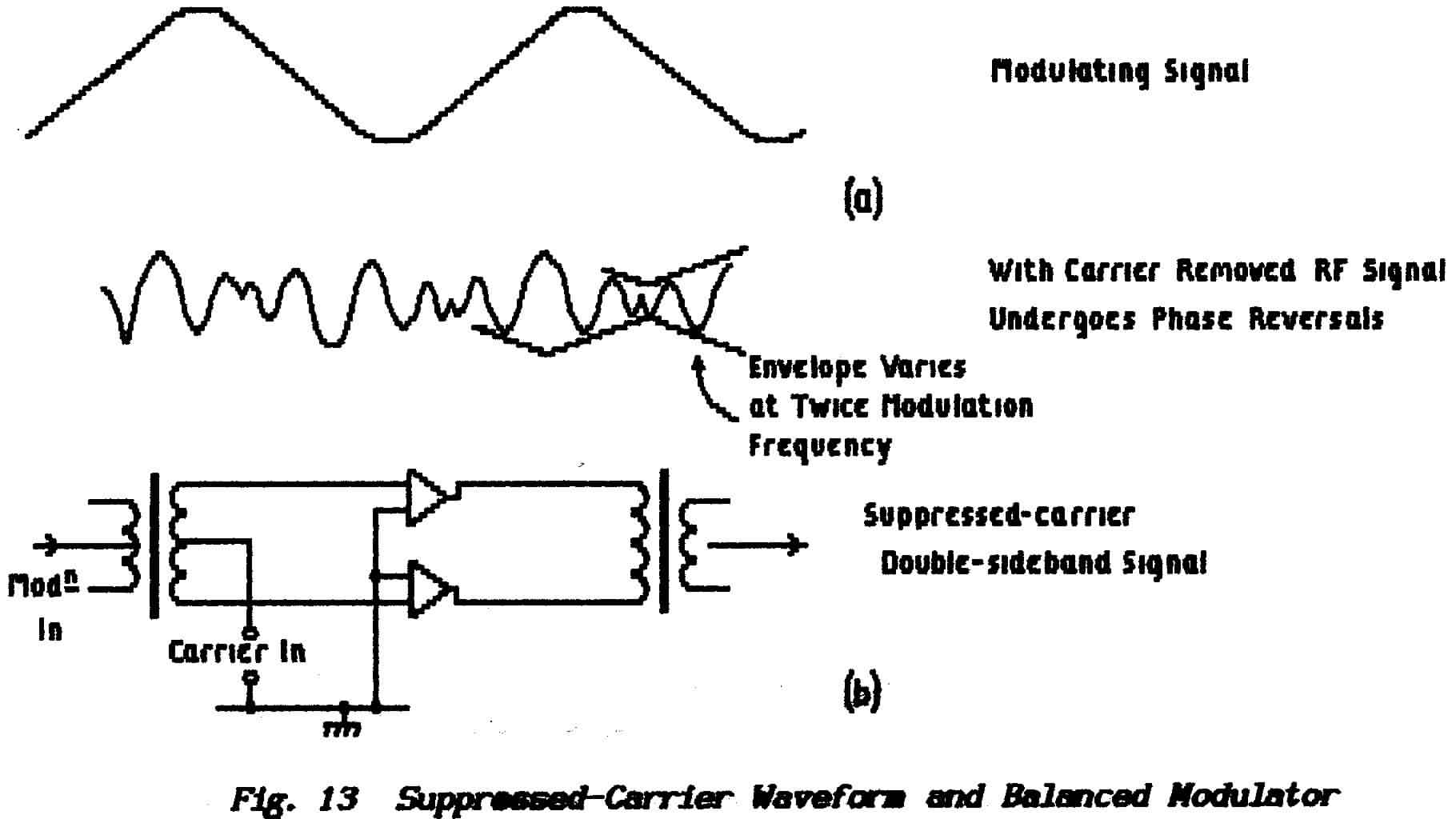
** The first stage in achieving ssb-operation is to produce an amplitude-modulated carrier but with the carrier itself suppressed. The signal which results from this is illustrated in Fig. 13(a); with each successive half-cycle of the modulating waveform the carrier suffers on abrupt reversal of phase. One circuit capable of this is the balanced modulator shown in Fig. 13(b).
>>>>>>>>>>>>>>>>>>>>
PAGE 25
<<<<<<<<<<<<<<<<<<<<
** The arrangement offers two signal paths into which the rf-carrier signal is fed in push-push so that, at the output, the two carrier signals cancel. The modulating signal is fed in push-pull so that it upsets the balance between the two carrier paths and allows carrier to appear at the output first through one side and then through the other. When combined in the output transformer the result shows the phase-reversals which characterise the double-sideband suppressed-carrier signal.
** Finally, to arrive at a single-sideband suppressed-carrier signal, the output from a balanced modulator is passed through a filter; depending on the design of this filter it eliminates either the upper sideband or the lower sideband.
** The advent of small semiconductor diodes has made possible the Ring Modulator. This uses four diodes connected in a ring formation in such a way that they act as a balanced modulator. This circuit arrangement has a variety of uses including the demodulation of ssb signals. These circuits are described in Part 5 of this Course but a detailed knowledge of their working is not required for the R.A.E.
(c) Modulated Oscillator
Any of the methods of amplitude-modulating an rf-amplifier can be applied directly to an oscillator thus producing a relatively simple transmitter. Skilful design, construction, alignment and operation can result in successful use of such but the practice is to be deprecated.
The need for sufficient bandwidth to handle speech signals limits the Q-value of the resonant circuit; on the other hand, to achieve good frequency stability and a good waveform (i.e. a low harmonic content), a high Q-value is necessary.
Single-stage transmitters are found most often in CW-working particularly in so-called QRP working (output less than 5 watts); in these transmitters there is no alternative to keying the master oscillator. Frequency drift tends to occur whenever the key is either closed or opened mainly because the voltage of the auxiliary power-supply changes as the load-current varies with the keying. The "squeal" which often accompanies the start and finish of each dash or dot is known as chirp which, apart from being an illegal emission, is most irritating to read.
(d) Frequency Modulation
To vary the frequency of an LC oscillator it is necessary to vary the value of either the inductor or the capacitor. Variation of the inductor is possible by using a "saturating reactor"; this is a cored inductor which is provided with an extra winding through which the modulating signal is passed.
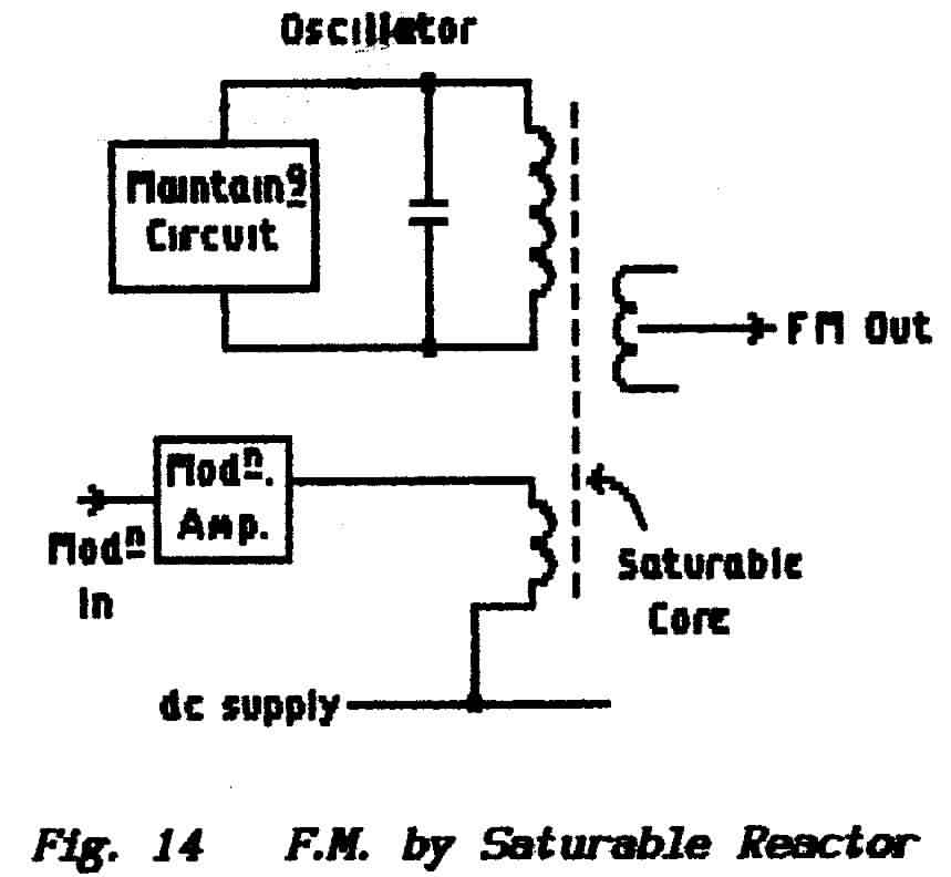 |
The magnetic field which accompanies the modulating signal increases and decreases the magnetic saturation of the core and so changes the inductance value. Magnetic devices however are not very linear and it is difficult to design good audio modulators in this manner. A typical circuit arrangement is shown in Fig.14; because the modulation signal is an ac it is effectively turned into a varying dc by adding dc-bias. |
>>>>>>>>>>>>>>>>>>>> PAGE 26 <<<<<<<<<<<<<<<<<<<<
Before semiconductors, F.M. was achieved by use of the Reactance Valve. This is an amplifying stage with negative-feedback applied directly from output to input via a capacitor. The 900 phase shift which the capacitor introduces into the feedback path results in the input of the stage appearing as a large capacitor whose value is the feedback-capacitance multiplied by the stage gain. Thus, if the modulating signal is applied so as to vary the stage gain, the input-capacitance of the stage varies accordingly. Such a circuit, when connected across the tuned circuit of an LC oscillator, results in frequency-modulation. See Fig. 15(a).
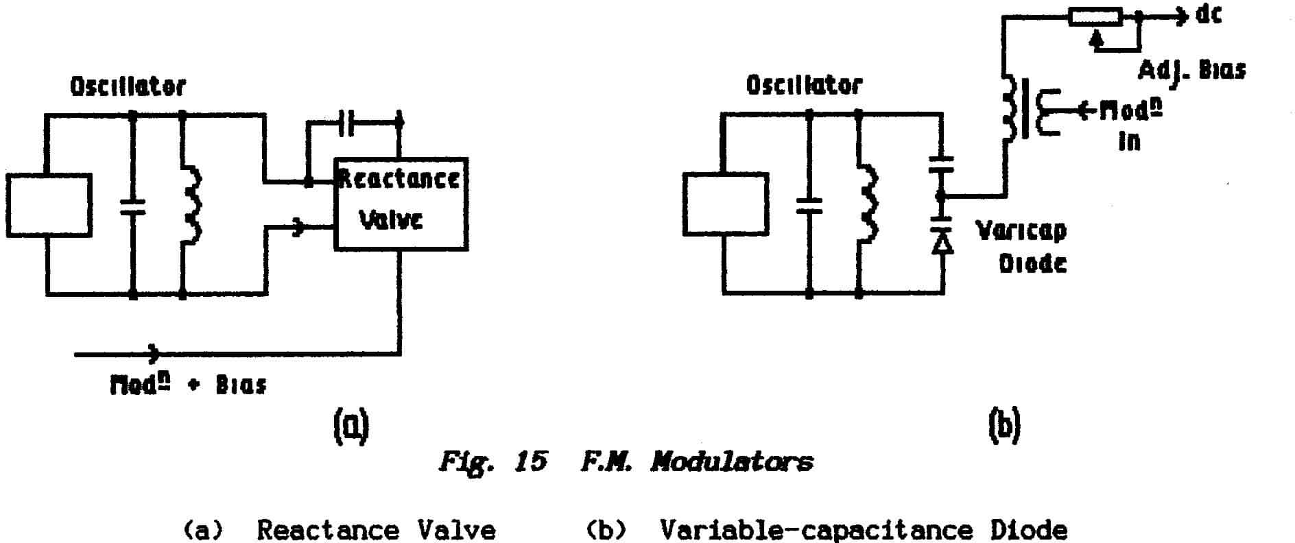
** The method works less well with transistors because of the large capacitances inherent in transistor construction. The more-usual F.M. modulator uses the variable-capacitance diode or Varicap; these are manufactured to exploit the fact that reverse-biased semiconductor diodes exhibit a capacitance which varies with the applied voltage. Connected across a resonant circuit these diodes are used both for F.M. modulating, as shown in Fig.15(b), and for non-mechanical tuning.
RC oscillators produce the necessary phase-shift effects by using networks of resistors and capacitors only . These can be modulated in similar fashion either by use of a variable-capacitance diode or by using a valve or transistor as a variable resistance.
(e) Phase Modulation
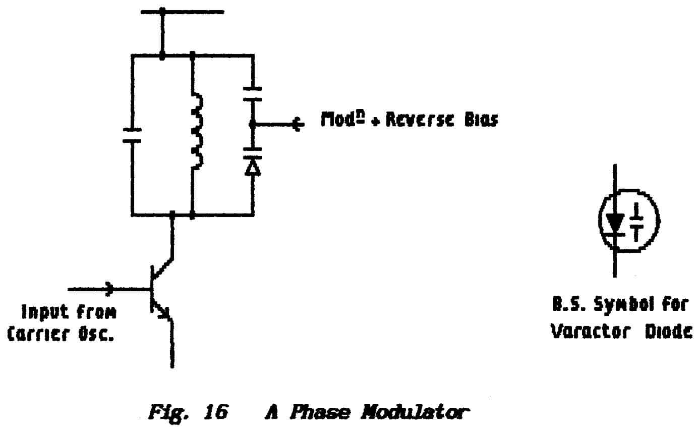
Resonant LC circuits are characterised by a rapid change of phase between applied voltage and circulating current as an applied signal passes through the resonance frequency of that circuit. This in fact is the mechanism which controls the frequency of a maintained oscillator.
The argument can be applied in reverse; if the frequency is maintained constant but the resonance-frequency of the circuit is varied there will be phase changes that follow the form of the tuning-changes.
This is the basic mechanism used to achieve phase-modulation and it is illustrated in Fig. 16. Here the resonant circuit is de-tuned by the variable capacitance but the circuit is driven by the constant frequency from a M.O.
>>>>>>>>>>>>>>>>>>>> PAGE 27 <<<<<<<<<<<<<<<<<<<<
(f) Mixed Modulation
** Varying the tuning of a resonant circuit as described in the modulating arrangements above also changes the circuit impedances and so causes a certain amount of amplitude modulation in addition to the F.M. or Ph.M. Similarly the circuits described to achieve A.M. often produce some F.M. (a bad example is the chirp from a keyed oscillator).
To overcome this effect F.M. and Ph.M. circuits are usually followed by some kind of limiting stage which removes the A.M. The only way to deal with unintentional F.M. in an amplitude-modulator is to take care with the design and construction so as to avoid the problem.
** The P.A. of a transmitter is the final stage of amplification in which the (perhaps modulated) radio signal is raised to the required power-level before it is passed to the aerial system where it will be converted to an electromagnetic wave. Note that the Amateur Licence restricts the maximum power level which may be radiated and that this level varies according to the Band in use; these limitations are laid out both in the licence document and in other literature and you are required to be familiar with them.
Because of the P.A.'s position "at the end" of a transmitter it is often known as the Final.
The detailed characteristics of tuned power-amplifiers are dealt with later under Electronic Amplifiers and in particular under the heading Class-A, Class-B and Class-C Amplifiers. The process known as "tuning-up" a transmitter consists of first setting the M.O. for the required frequency of operation and then adjusting the P.A. for maximum efficiency in its operation; the P.A. handles power and, unless it delivers that power efficiently to the aerial system, it will be destroyed.
Many transmitters have a Mode switch on which one position is marked "Tune". In this position the P.A. is specifically restricted in its ability to draw power and so it becomes possible to make the necessary adjustments without fear of damage. Once these adjustments are completed the switch is returned to the "Normal" position and then, carefully, the final adjustments are made on full power.
>>>>>>>>>>>>>>>>>>>> PAGE 28 <<<<<<<<<<<<<<<<<<<<
** While making such adjustments considerable interference can be caused to others already working around the chosen frequency and so setting-up procedures should be carried out with the transmitter connected to a dummy load. This is simply a screened and ventilated resistor, usually of 50-ohms, that is capable of handling the transmitter output without overheating. For setting up of course it need handle only the reduced power but full-power tests should not be made using an aerial - unless the object is to test the aerial.
There is another reason for using a dummy load which is of especial importance when using a transmitter fitted with a transistor P.A. Part of the necessary adjustments are concerned with achieving a proper match between the P.A. and the aerial system (see under 1.12.5: Impedance Matching). Failure to match properly makes it impossible for the P.A. to transfer power to the aerial system and the large voltages and/or current-demands that result can easily destroy a transistor P.A. Valves are fairly robust and, within reason, will withstand a mismatch but it is not good engineering practice to use transistors in a P.A. for other than low powers.
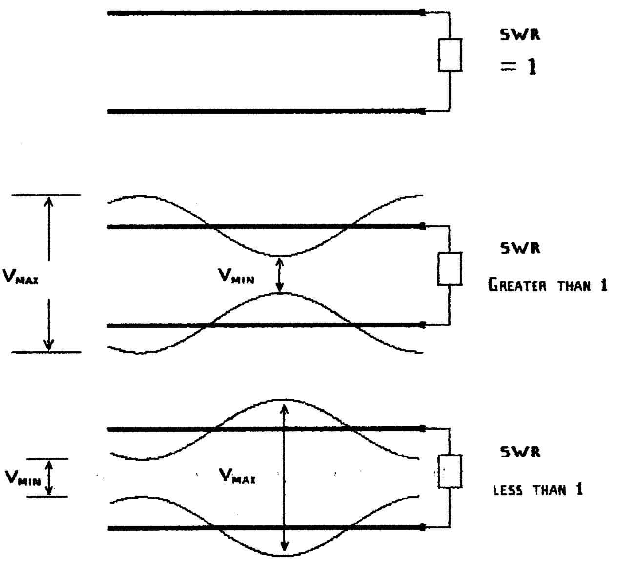
A further complication arises in that an aerial is unlikely to provide a good match to its feeder except at a few spot frequencies and this results in the appearance on the feeder of a standing wave which is explained in the next Section. Standing-wave problems can be overcome by use of a so-called Aerial Tuning Unit (ATU) but, until this unit has been properly adjusted, there is again a risk of destroying a P.A. Note: the name Aerial-tuning Unit is a misnomer because the one thing which the unit does NOT do is tune the aerial! (The initials really stand for Aerial Transducer Unit where a transducer is a device which changes the form of energy; e.g. an electric motor is an electro-mechanic transducer.)
** A P.A. should unload its power into an aerial in the form of the intended radio signal but it is possible for part of that power to appear in the form of spurious signals . These can be harmonics of the carrier and of the side-frequencies caused perhaps by over-modulation or they might be unintended oscillations which can appear on unexpected frequencies. Additionally some of these frequencies may beat together to form sum-and-difference frequencies or they may even beat with transmissions from other stations. It is a requirement of the Amateur Licence that transmitting equipment is checked regularly to ensure that such emissions do not occur and all such tests should be recorded in your Log. See also under Filters.
WARNING
The P.A. in particular is the part of a transmitter where danger lurks for the unwary . With valve P.A.'s the auxiliary supply may operate up to 1,000 volts and be capable of supplying a half-amp which most definitely IS LETHAL. Transistor P.A. s seldom require more than 50-volts but, under some conditions, even 50 volts can kill.
Never wear a wristwatch with a metal strap when going inside a P.A. or any other semiconductor equipment; the low-voltage supply will be capable of producing many amps which will make that wrist-strap red-hot in a contact of seconds.
Large rf voltages and circulating currents can be encountered, especially in ATU's, which can be just as lethal. Additionally rf burns cause serious damage to skin structure and so take a long time to heal as well as being extremely painful.
>>>>>>>>>>>>>>>>>>>> PAGE 29 <<<<<<<<<<<<<<<<<<<<
** At the output from a transmitter the P.A. should produce only the carrier signal and those side-frequencies which arise as a consequence of the intended modulation. In practice however there is likely to be also harmonics of the carrier, of the side-frequencies arid other so-called spurious signals. There could also be cross-modulation products which are the sum-and-difference frequencies which result when all these signals beat with each other.
** Harmonics of both carrier and modulation frequencies arise naturally from non-linearities (imperfections) of the various active devices used in the amplifying stages but harmonics of the side-frequencies arise specifically through over-modulation. All signals whose frequencies are greater than the highest legitimate side-frequency can be eliminated by use of a low-pass filter (L.P.F.) but unintended side-frequencies which are below the carrier frequency cannot.
** A low-pass filter is a network of inductors and capacitors which has negligible effect on the passage of signal currents up to a given frequency; above that frequency (the cut-off frequency) signals are increasingly attenuated. Such a filter, placed at the very output of a transmitter between the P.A. and the feeder, eliminates the risk of inadvertently radiating spurious signals which are above the legitimate transmitting range. Harmonics of the modulating signal which have been produced either before the modulator stage or during the modulation process produce their own side-frequencies both above the carrier and below it; these lower-sideband frequencies cannot be stopped by the L.P.F.
** Protection from emissions below the carrier requires the use of more expensive bandpass filters (B.P.F.) which, as the name implies, have a lower as well as an upper cut-off frequency. Good engineering practice - and common sense - dictate that equipment should be properly adjusted so that modulation-signal harmonics are not generated.
** Probably the major cause of this type of distortion is abuse of the so-called speech processor with which most modern transmitters are equipped. The idea is to amplify the speech signal so that the quietest sounds fully modulate the transmitter; all signals of greater strength are then reduced so that over-modulation does not occur and the transmitter always produces maximum modulation which results in maximum information-power.
** The best way to achieve this aim is by use of a Limiter which is a variable-gain amplifier whose gain is adjusted by the signal level (a feedback arrangement). A cheaper and so favoured method is to amplify the signal but then to clip the waveform at a pre-determined level by means of a diode ; this of course causes serious waveform distortion which is then removed by use of an audio low-pass filter. Such processors or compressors work well provided that the amount of speech compression is limited ; beyond a certain point they render the speech characterless and emphasise breathing noises. Eventually speech is degraded into a series of thumps and becomes all but unintelligible.
** Filters at the output of a transmitter come in a variety of guises. One obvious LC circuit is the resonant circuit which forms the load of the final amplifier ; see under Electronic Amplifiers. In fact this is a bandpass circuit but its performance as such may not give much protection. It has been mentioned already that this circuit exists to lose power to the aerial system and so operates with a relatively-low Q-factor. Nevertheless it can be arranged so that it acts also as a L.P.F. the most famous form of which is probably the P1 Tank Circuit. This is discussed in detail later and it is sufficient to note here that the
>>>>>>>>>>>>>>>>>>>> PAGE 30 <<<<<<<<<<<<<<<<<<<<
inductor is placed in series with the signal path to the aerial while the capacitor, divided into two discrete parts, is arranged to shunt the signal path to ground. Because the circuit is resonated at the carrier frequency it does not attenuate the carrier and its sidebands.
** The P1 circuit illustrates another function often fulfilled by an output filter namely impedance matching. Under 1.10.4 it was shown that a tapped inductor acts as a single-wound transformer (an autotransformer). In a resonant circuit a similar facility can be obtained also by tapping the capacitive leg; i.e. the tuning capacitor is split into two or more discrete capacitors as is seen in the PI circuit.
**Another filter arrangement increasingly seen at the output is the misnamed ATU (aerial-tuning unit) . An aerial can be constructed and adjusted so that it matches the impedance of its feeder but only at one frequency. It is possible to obtain a good match at several spot frequencies so producing nominally "wide-band aerials" but effective matching over a continuous band of frequencies is not possible. Amateur aerials are required to operate with bandwidths up to 10%. of centre frequency over several harmonically-related Bands.
** The result of a mismatch between aerial and feeder is that, when in use for transmitting, a standing-wave appears on the feeder (see next Section). This means that, at the other (transmitter) end of that feeder, the impedance presented to the transmitter varies with frequency. The purpose of the ATU is to provide continuously-variable correction so that, whatever operating frequency is chosen, the feeder impedance can be matched to the P.A.
** An important point not generally realised is that an ATU does NOT remove the standing wave on the feeder; to remedy that either the aerial must be made to match the feeder or the ATU must be placed between the aerial and the feeder. This is not a practical arrangement because it requires servo-systems to adjust the ATU controls and a weatherproof casing.
** Few ATU circuits provide attenuation of harmonics and a separate L.P.F. should always be used.
END OF LESSON 5
* * * * * * * * * * * *
QUESTIONS
1. Impressing information on to a carrier wave by amplitude-modulation increases the total carrier power. Why is this and from where is the additional power drawn ?
2. What is the advantage of single-sideband operation ?
3. Give a brief description of the manner in which frequency modulation is achieved usually in modem equipment. Why is such a circuit usually followed by a limiter stage ?
4. Describe the purpose of the "Tune" mode in a transmitter
5. Why is a dummy load an essential piece of transmitting equipment ?
6. Why are filters used at the output of transmitters ?
7. An Inductor of 0.5 Henrys has a dc-resistance of 12 ohms and is connected in parallel with a resistor of 6,000 ohms. What is the impedance of the combination at 1 kHz ? Make reasonable practical approximations.
>>>>>>>>>>>>>>>>>>>> PAGE 31 <<<<<<<<<<<<<<<<<<<<
(Only paragraphs marked ** are required for the R.A.E.)
** A transmission line is a system of conductors which is used to transfer electrical energy from one point to another. An everyday example is the overhead Grid distribution system of the Electricity Boards but we are concerned here with the transfer of rf-power from a transmitter to an aerial system or from that aerial system to the input of a receiver. Such transmission lines are often called feeders.
** Usually a feeder consists of a pair of conductors which are arranged:
(a) straight and parallel held apart by "spreaders" (an open-wire feeder),
(b) twisted together (a twisted pair)
(c) placed co-axially one within the other.
Feeders which handle very high powers may consists of four conductors in open-wire form with the diagonally-opposite conductors connected in parallel.
The energy is actually carried in the electro-magnetic field (e-m) field which travels between the conductors; it is supported by the voltages between the conductors and by the currents which flow on the surfaces of those conductors. In a coaxial line this e-m field is completely enclosed by the outer conductor and so is less likely to cause unintentional radiation or to be influenced by incident e-m radiations (noise).
For technical theoretical reasons waveguides, used at extremely high frequencies, are not classified as transmission lines but they can be viewed as coaxial lines with the centre conductor removed which does demonstrate that the flow of energy is contained in the traveling e-m field. It is possible too at these frequencies to make a waveguide from a tube or rod of dielectric material without conductors or from a single conductor which is thinly coated with a dielectric material.
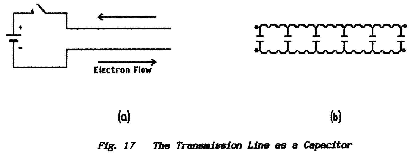
Under 1.7.2 in Lesson-2 of Fundamentals-1 the capacitance of a capacitor was stated to be a function of plate area and of plate separation and not to depend in any way on the shape of those plates. Thus a transmission line can be regarded as a capacitor which has been constructed from two very long and thin plates. Fig. 17(a) shows such a capacitor connected to a cell via a switch.
When the switch is closed the capacitor can be expected to charge as discussed previously. However, the capacitor discussed in Lesson-2 of Fundamentals-1consisted of two square plates with the connections taken to their centres; here, with the connections made at one end, electrons have to travel the length of the narrow plates as they either enter the capacitor or leave it. Such a movement of electrons constitutes a flow of current ; that current takes a real (or finite-length of) time to travel from one end of the transmission line to the other.
>>>>>>>>>>>>>>>>>>>> PAGE 32 <<<<<<<<<<<<<<<<<<<<
Under 1.9 in Lesson 4 of Fundamentals-1: Induction, Inductors and Inductance it was shown that conductors which carry current interact with a surrounding magnetic field to produce Inductance whereby changes of current-flow are opposed. The transmission line therefore must be more than just a long thin capacitor; electrons cannot move freely along the line but are impeded by the inductance of the conductors.
(a) Path of Electrons During Charging
(b) Representation of Electron-path Inductance
Fig. 17(b)shows an attempt to represent this by drawing the conductors as long Inductors which are connected at regular intervals by a series of small capacitors. However the diagram is not correct because the real line capacitance is not divided into a number of discrete components but is distributed evenly along the line as are the inductances. For this reason a transmission line is said to possess distributed inductance and distributed capacitance as distinct from the lumped inductance and lumped capacitance of discrete manufactured components.
Nevertheless the distributed inductance does have the effect of isolating small sections of distributed capacitance in that it delays the passage of electrons from section to section as the line attempts to charge from the cell. In fact an artificial line can be constructed from discrete inductors and capacitors as shown in Fig.18 and the arrangement does indeed behave in the manner of a transmission line. Although such a device is not employed to convey power it can be used for example to delay the passage of a signal between two points and then it is known as a delay line.
When the switch is closed the terminal voltage of the cell and the terminal voltage of the input-capacitor C1 become identical; the capacitor however is not charged and so the cell-terminal voltage has to fall to zero.
With zero voltage across the line current cannot flow into it via inductors L1a and L1b and so the entire current from the cell must flow into C1. As the capacitor charges so a p.d. begins to build-up between its terminals which
>>>>>>>>>>>>>>>>>>>> PAGE 33 <<<<<<<<<<<<<<<<<<<<
(a) opposes the flow of current into C1 and
(b) begins to drive a current into the line through distributed inductances L1a and Llb
However, as discussed in Fundamentals-1, the nature of inductors is to oppose any change in the rate of current-flow and so the introduction of charge to distributed-capacitance C2 is delayed.
As a repeat of the last two paragraphs - current cannot flow into the transmission line beyond C2 until that capacitor has acquired an accumulation of charge and the inductive effects of L2 have been overcome.
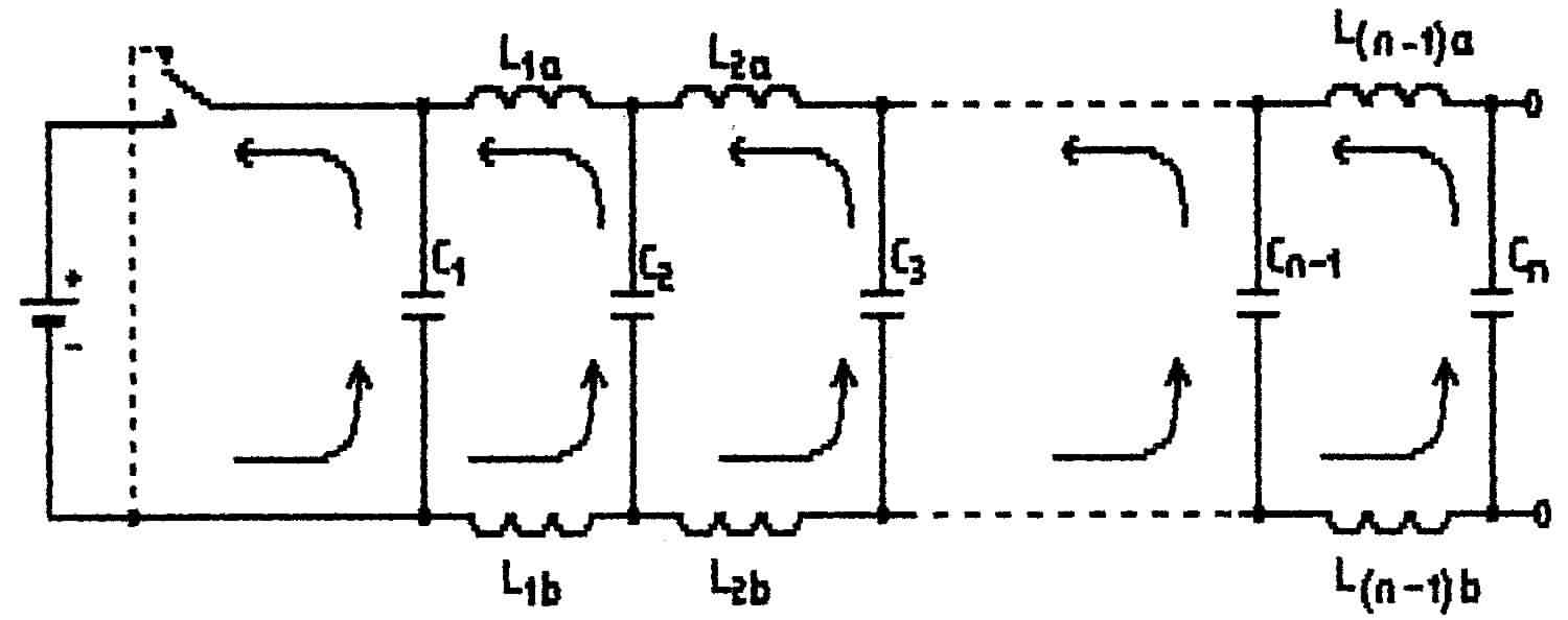
Fig. 18 Artificial Transmission Line
There are several points of interest in this line-charging action:
(i) Current does not flow instantly along the length of the transmission line when the switch is closed. Time is required for the current to steeplechase its way from section to section constantly delayed by the distributed inductance (which resists the build-up of current) and by the distributed capacitance (which delays the build-up of voltage).
This is expressed in technical language by saying that a wavefront propagates along the line; a wavefront in which current begins to flow in the line and charge begins to accumulate in its distributed capacitance. This is shown graphically in Fig. 19 where the right-hand side of the curve shows the changing value of current as the wavefront passes along the line. Because this is the first wavefront to pass down the line it is referred to as the leading wavefront.
>>>>>>>>>>>>>>>>>>>> PAGE 34 <<<<<<<<<<<<<<<<<<<<
(ii) When the wavefront reaches the far end of the line what happens depends on what is connected at that end. If the line is open-circuited then the final capacitive section charges to the value of the emf and the line current falls to zero.
If the line is short-circuited at the far end then the final capacitive section fails to charge and the line current reaches a value equal to the emf of the cell divided by the internal-resistance of the cell.
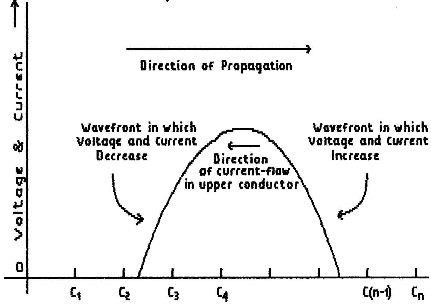
Fig. 19 Charge and Discharge Wavefronts with DC Excitation
If a load is connected then the final values of line current and line voltage must settle in the ratio defined by Ohm's Law for that load.
(iii) At the moment the wavefront is launched into the line the p.d. across the line begins to rise and so too does the line current. This can continue only for a short time because the line current, flowing through the cell's internal resistance, must limit the terminal voltage to a value less than the cell's emf.
We can conclude therefore that, if the transmission line is very long, the ratio of line-voltage to line current at the input will stabilise before the last sections of the line have begun to charge (before the leading wavefront arrives at the far end). This combination of line-voltage and line-current has nothing whatever to do with any load which may be connected at the far end ; it is determined only by the distributed-inductance and distributed-capacitance of the line.
>>>>>>>>>>>>>>>>>>>> PAGE 35 <<<<<<<<<<<<<<<<<<<<
(iv) There is a mischievous thought "What happens if, when the leading wavefront is only half-way along the line, the switched is opened ?
Although the cell is no longer available to supply the line current the distributed inductance resists any fall in the current value ; this continuing current-flow can be obtained only by discharging C1 and the current in L1 will fall gradually to zero as the capacitance is discharged.
This action is then repeated discharging first C2, then C3 and so on along the line. Thus a second discharging (or trailing) wavefront propagates down the line.
Between the leading and trailing wavefronts there now exists the strange phenomenon of a short pulse of direct-current which is traveling along the line toward the load end. Note that this voltage/current relationship is not influenced in any way by a connected load (which, as yet, is not aware that a generator has been connected to the line) nor by the cell which, after causing all the commotion, has now been disconnected from the line.
Of particular interest is the fact that the dc-pulse continues to travel toward the load when it might be expected to spread evenly along the line. Had the cell been connected to the centre of the line, and then disconnected again, the input current would have divided and flowed in both directions but the end result would have been two pulses traveling in opposite directions.
It is the presence of distributed-inductance and distributed-capacitance which keeps current flowing once launched into the line and prevents the accumulated charge from spreading evenly throughout the distributed capacitance.
(v) The last point of interest arises from the different possibilities of a connected load:
(a) Not Terminated
Without a connected load the final capacitive section of the transmission line in Fig. 18 is denied a discharge path. Thus, because the distributed inductance maintains the current-flow, so this final capacitive section must acquire the entire charge that was delivered by the cell. It can be shown mathematically and practically that, at the moment when current finally ceases, the final capacitive section is charged to a value twice that of the line-voltage between the two wavefronts. (This final value is greater than the emf of the cell; it can be shown that equal power is carried in the electric and magnetic field).
The final cessation of line current signals the end of the inductive effects that kept the current flowing toward the load end of the line. Thus the final capacitive section is now free to discharge back into the line so causing a flow of current toward the cell. As this section becomes discharged however it simulates the original action of opening the switch and so a new dc-pulse appears traveling toward the cell end of the line.
>>>>>>>>>>>>>>>>>>>> PAGE 36 <<<<<<<<<<<<<<<<<<<<
Although this return pulse is a new pulse re-constituted from the stored charge it is usual to regard it as the original pulse reflected from the open-circuited end of the line. Note that, when reflected from an open-circuit, the pulse retains the same polarity but the direction of current flow on the line (and the direction of propagation for the pulse) has been reversed.
The reflected pulse travels to the input end of the line where the switch is open and so suffers a second reflection from an open-circuit. In fact it must continue to bounce up and down the line but it slowly decreases in amplitude because its energy is dissipated as heat in the resistance of the conductors.
(b) Terminated by a Short-circuit
Referring again to Fig. 18 a short-circuit termination means that the final capacitive-section represented as Cn cannot charge. When the leading wavefront arrives at the end of the line the inductive effect causes current to flow through the short-circuit from (as shown) the lower conductor to the upper conductor. As this current-flow continues so the penultimate capacitive-section Cn-1 becomes first discharged and then recharged with opposite polarity.
Once again a "reflected pulse" appears propagating toward the input end of the line but with a difference. This pulse, reflected from a short-circuit, has reversed polarity but retains the same direction of current-flow. Again this corresponds with the reversed direction of propagation for the pulse.
When this pulse suffers re-reflection at the open-circuited input end of the line it retains its polarity but undergoes a reversal of current as before and conditions on the line become complicated until the pulses have been dissipated. If required this can be averted by arranging the switch so that, when it disconnects the cell, it shorts the transmission line ; can you draw such an arrangement ?
(c) Resistive Termination
A resistor connected across the line allows current to flow between the two conductors but restricts its value ; at the same time it develops a p.d. across the final capacitive section. This modifies any reflected pulse mainly in its amplitude with respect to the incident pulse ; it also dissipates quickly the energy of reflected pulses.
There is a value of resistance however which will support the ratio of current to voltage which exists on the line between the two wavefronts. If such a resistance value is used as a termination then the energy of the incident pulse is utilised completely in heating the resistor without disturbing the voltage/current relation ; current-flow does not cease until the distributed capacitance is fully discharged and so reflected pulses do not appear.
The value of resistance which supports the same voltage/current ratio as does the transmission line is known as a matching load; a line which does not produce reflections is said to be matched. This ratio of voltage/current which exists within the dc-pulse, irrespective of input or load conditions, is referred to as the characteristic resistance of the
>>>>>>>>>>>>>>>>>>>> PAGE 37 <<<<<<<<<<<<<<<<<<<<
transmission line; thus a line is said to be matched and fails to produce reflections when it is terminated in a resistive load equal to its characteristic resistance.
There are two practical points worth noting. All transmission lines have resistance and so dissipate energy as heat; thus, as a pulse propagates along the line, it slowly decreases in amplitude. If a line is sufficiently long it will totally absorb a pulse before it reaches the load end. Under these conditions a reflected pulse cannot appear whatever the load may be. Even for a shorter line it may be that the return length (to the far end and back to the input end) is sufficiently long to totally absorb a pulse ; thus, although a reflected pulse may be generated, it will not appear at the input.
** In both instances an observer might conclude that the load was absorbing the power and so the line must be matched. Thus an infinitely (or sufficiently) long line will behave as a resistance equal to its characteristic resistance independent of its terminations.
** The second point is that the characteristic resistance is determined by the ratio of distributed inductance to distributed capacitance and, in turn, these are determined by the physical dimensions of the line . Thus the characteristic resistance of a line is controlled by selecting the diameter of the conductors and the spacing between them.
END OF LESSON 6
* * * * * * * * * * * *
QUESTIONS
1. What is the reason for the somewhat strange behaviour of electric charges on a transmission line ?
2. A pulse is traveling along a transmission line ; why does it continue to travel as a pulse rather than disperse its charge evenly throughout the length of the line ?
3. The characteristic resistance of a transmission line is not at all connected with the dc resistance of its conductors ; what determines this characteristic resistance ?
4. A positive-going pulse is reflected from the open-circuited end of a transmission line. Describe the reflected pulse.
5. What are the two conditions on a transmission line each of which would result in the non-return of a pulse to the input end ?
>>>>>>>>>>>>>>>>>>>>
PAGE 37(again)
<<<<<<<<<<<<<<<<<<<<
When a transmission line is connected to an ac source the result, at first, is the same in that a leading wavefront is launched into the line in which current rises, and charge accumulates, in the distributed capacitance.
The intervention of a switch is not required here however because the ac-source reduces the applied voltage to zero and then reverses the polarity. Hence the second wavefront becomes one in which the distributed capacitance is first discharged to zero but then re-charged with opposite polarity ; at the same time the line current also falls to zero and builds-up again but flowing in the reverse direction. This is illustrated in Fig. 20.
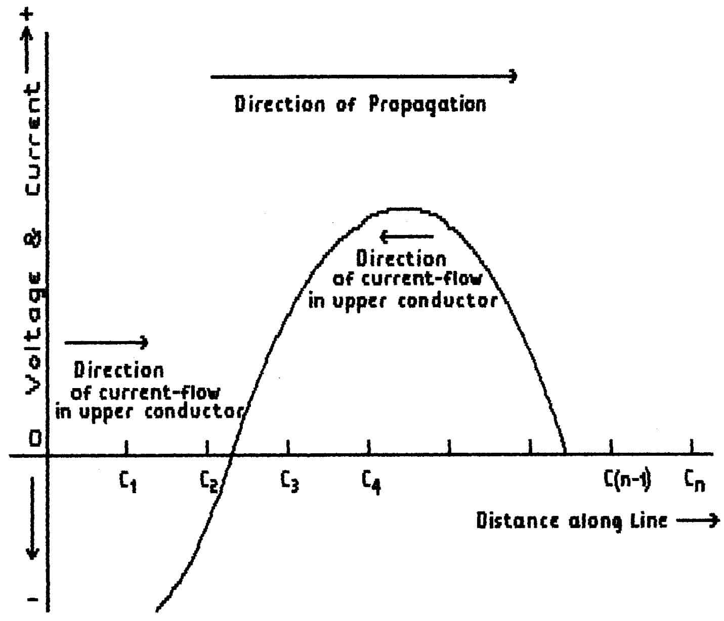
Fig. 20 Charge and Discharge
Wavefronts With AC Excitation
Note that, in the second wavefront, both current and voltage reverse direction and the wavefronts continue to propagate toward the load end of the line.
There are two major differences in the line behaviour when the source is changed from dc to ac:
(i) with a dc-source (reference Fig. 18), charge is transferred continuously along the line from C1 to C2 to C3 ... With an ac-source, because the line current constantly reverses, the charge flows back and forth along the same section of line ; e.g. from C1 to C2 and then back to C1 .
>>>>>>>>>>>>>>>>>>> PAGE 38 <<<<<<<<<<<<<<<<<<<<
(ii) the leading wavefront and the following wavefront now define a section of line in which current-flow occurs in both directions toward a point of zero current. This point of zero current is associated with a point of zero voltage where the waveform changes polarity.
This entire configuration repeats as the source cycles and it travels along the transmission line away from the source ; this moving pattern is referred to as a traveling wave.
In the transmission line driven by an ac-source electrons oscillate back and forth along a short path but the magnetic and electric patterns (fields) which they create travel continually toward the load. It is the combination of these two traveling fields that carries the power along the line (power requires both voltage and current).
At the end of the transmission line, if a matching load is connected, the ratio of voltage-to-current (as represented by the electric and magnetic fields) can be maintained and so the power is totally absorbed by the load and dissipated as heat. Note that current minima are coincident with voltage minima ; i.e. the current and voltage waveforms are in phase which means that the line is behaving like a resistance - its characteristic resistance.
If the connected load is anything other that the characteristic resistance then, as with the dc-source, the load cannot absorb all the power and there is a residual alternating-current or alternating-voltage which is re-launched back down the line. The two traveling alternating-waves, one moving toward the load and the other moving back toward the generator, are otherwise identical and they interfere to form a distinctive cyclic pattern which does not change provided the conditions remain constant.
This fixed pattern is known as a standing wave and it differs from the traveling wave in that it is not truly a wave pattern at all ; it has the nature of a graph which illustrates the amplitude (the size) of alternating current-flow or alternating voltage at successive points along the line . The electric-field graph is not in phase with the magnetic-field graph . This implies that the line is behaving in the manner of a reactance and is carrying a certain amount of wattless current ; this is not surprising when the load is failing to absorb all the power that (apparently) is being injected by the source.
** It is not necessary to analyse the line behaviour in detail for the RAE but the following points are important to grasp. There are places at regular intervals along a mismatched line where the line-voltage is high but the line current is small; at such points the line is presenting a high impedance. Mid-way between these places there are others where the line-voltage is low but the line-current is large; at such points the line is presenting a low impedance.
** Should one of these points of high voltage fall at the input terminals of a receiver then the voltage-waveform of the incoming signal will be enhanced: should one of the points of low voltage fall at the input terminals of a receiver then the voltage-waveform of the incoming signal will be degraded. However, should a point of high voltage or high current-demand fall at the output terminals of a transmitter then there is considerable risk of damage occurring to the P.A. stage. For this reason it is most important that a transmitter be connected only to a matched line.
>>>>>>>>>>>>>>>>>>>> PAGE 39 <<<<<<<<<<<<<<<<<<<<
There is advantage when receiving in having a ms-matched aerial system such that a point of high-impedance occurs at the receiver input but successful use of this ploy requires two independent aerials. This is not a practical objective when using a Transceiver(a piece of equipment that is switched to serve alternately as a transmitter and then as a receiver) ; a single-aerial system as required by a transceiver must be properly-matched.
For those not happy with the above explanation of a standing-wave the following may help . The concept of power being reflected from a mismatching load is a powerful way of explaining to students the queer things that happen on a transmission line . Indeed , if power is applied to a line as a train of rf-pulses, then the forward and reflected pulses can be viewed on an oscilloscope.
Do not take this explanation too far ; it does not work for continuous-wave signals. For example consider power derived from a transmitter and reflected from a mismatched load ; where does that power go when it arrives back at the transmitter ? It cannot be absorbed by the transmitter . If it is re-reflected then the transmitter must reduced its output by the amount of that reflected power else even funnier things must happen ?
The voltage/current ratio dictated on the line by the distributed L & C is not supported by a so-called mismatched load ; the ratio must change . The situation is analogous to that discussed in connection with real and apparent power involving a power factor ; where a product of voltage x current does not correspond to the amount of power being dissipated there must be a power-factor involved which means that the current and voltage must depart from being in-phase (see Fundamentals-1, Lesson-7) The lack of synchronism between voltage and current coupled with the distributed L & C gives rise to the amplitude-variations that constitute a standing-wave.
It was stated above that the patterns of voltage and current on a mis-matched line are not in phase and so such a line behaves like a reactance; by contrast a matched line behaves as a resistance.
** Along the length of a mis-matched line the impedance constantly changes cycling between capacitive reactance and inductive reactance ; at points approximately a quarter-wavelength apart the reactance changes sign and here the line becomes purely resistive. Such points of resistance alternate between being greater than the characteristic resistance and less than the characteristic resistance. Thus a length of transmission line with well-chosen characteristic resistance can be used as a high-frequency transformer ; it is cut to be a quarter-wavelength at the required frequency and so supports at one end the lower of the two impedances to be matched and, at the other end, the higher of the two impedances. A more convenient way of achieving this is given in the next paragraph.
** Short lengths of transmission line are used also to correct the driving-point impedances of aerials; these are known as stubs. Cut either longer or shorter than a quarter-wavelength they provide an inductive reactance or a capacitive reactance that is connected either in series or in parallel with an aerial to make it appear purely resistive. A quarter-wavelength long transmission-line (a quarterwave transformer) can then be used to transform this resistive value to that required for matching to a feeder.
>>>>>>>>>>>>>>>>>>>> PAGE 40 <<<<<<<<<<<<<<<<<<<<
** A standing-wave pattern is related to the frequency of the rf-signal in that it repeats with each successive cycle. However the wavelength of the pattern in a feeder is shorter than that calculated for a radiating e-m wave because the distributed reactances of a transmission line delay the propagation. The ratio of the two rates of propagation is expressed as a velocity ratio or velocity factor whose value is obtained from data issued by the manufacturer and this has to be taken into the calculation when cutting the required length.
Short lengths of transmission line are used also as reactors and as resonant circuits in rf amplifiers, oscillators and insulators. They are particularly useful at frequencies above 100 MHz where normal lumped reactors become impossibly small.
** The appearance of a standing-wave on a transmission line which is fed with ac indicates that a mismatch exists at the receiving end of that feeder. For example a standing-wave on a feeder that is carrying power to an aerial shows that the driving-point impedance of the aerial does not match the characteristic impedance of the feeder. A standing-wave on the same feeder which is connecting the same aerial to a receiver shows that the receiver input-impedance does not match the feeder impedance.
Although it is true that, in both instances, re-reflection must occur at the input-end mismatch it is a greater truth that a standing-wave cannot be generated at all unless there is a mis-match at the delivery point. This is the reason for saying that an A.T.U. is mis-named ; while it may be able to produce a good match between feeder and P.A. output it cannot remove the standing-wave on the feeder because this is caused by the mis-match between feeder and aerial. Note too that an ATU cannot be adjusted by tuning for maximum incoming signal .
** A standing-wave is an undesirable feature for several reasons:
(a) its cause is the failure of the load to absorb all the power that could be presented by the source - the system is acting inefficiently
(b) at points separated by a half-wavelength the line is subjected to excessive build-up of voltage which could damage the feeder
(c) at these points of high voltage the dielectric losses in the insulating material, which are proportional to the square of the voltage, can become excessive causing localised heating with possible failure of the feeder
(d) midway between points of voltage maxima there are points of current maxima where again localised heat-generation, which is proportional to the square of the current, could cause the feeder to fail
(e) failure to present the P.A. with the correct value of resistive load causes a loss of efficiency in that P.A. which, at the best, limits the output power which the stage can generate without self-destruction
>>>>>>>>>>>>>>>>>>>> PAGE 41 <<<<<<<<<<<<<<<<<<<<
(f) when a point of maximum voltage or of maximum current-demand appears at the P.A. terminals then damage is likely to result in the stage ; this is of particular importance where a P.A. employs semiconductor devices.
[Items (e) & (f) are the main reasons for employing an ATU in Amateur working ; in high-power systems which transmit several kilowatts items (b), (c)& (d) become significant also.]
** In practice it is not possible to eradicate a standing-wave entirely and a criterion is required for its assessment. A perfect match is indicated by the non-appearance of a standing-wave whereas a total mismatch (i.e. either an open-circuit or a short-circuit both of which produce a 100% reflection) results in both current and voltage waveforms varying between zero (complete cancellation) and twice normal amplitude.
** As the condition of perfect-matching is approached so the standing wave tends to disappear or, as it might be interpreted, the ratio of maximum to minimum values approaches 1:1 . With a total mis-match so the ratio of maximum to minimum values tends toward an infinite value.
** This standing-wave ratio or swr is used as an indicator of the quality of the matching. The ideal perfect match is often referred as a swr of 1:1 which is a bit of a puzzle to the uninitiated. In practice however it is not attainable. A swr of 2:1 is beginning to get serious on low-power installations such as Amateur rigs and really is serious with transistor P.A. stages. A ratio of 1.1 : 1 (or about 10%) is about as good a match as is possible if costs are to be kept within reason both in the equipment itself and in the measuring gear used to achieve that degree of matching. However the problem usually lies not so much in achieving a good match as in ensuring that the good match remains.
>>>>>>>>>>>>>>>>>>>> PAGE 42 <<<<<<<<<<<<<<<<<<<<
Fig. 20(A) Receiver System Gain |
In a transmitting system the ideal is 1: 1 because it indicates maximum efficiency and that all the power is being transferred to the aerial for conversion to a radiating e-m wave. In a receiving system however, as already mentioned, the perfect match is not necessarily the best objective. The feeder is made to support a standing-wave by ensuring that the input impedance of the receiver is greater than the characteristic impedance of the feeder ; thus a voltage maximum occurs at the receiver input. In this manner the feeder is made to provide a selective "voltage gain" (but it does not provide amplification). This neat little trick applies only to fixed-frequency working or to where the receiving equipment is required to cover only a small range of frequencies. Receiving installations operate only at microwatts and so the disadvantages of permitting a standing-wave, as listed above, do not apply. As a purely practical point however it should be noted that a swr of 1:1 cannot be achieved in practice and so every effort should be made to ensure that error in the input impedance of any receiver makes it greater than the characteristic impedance of the feeder to which it is connected . Should the input impedance be less than the characteristic impedance then the feeder will provide a voltage-loss. |
Although swr is loosely defined as the ratio of maximum to minimum values this is only part of the story because, expressed in this way, it does not reveal whether the mismatch is too high or too low. Where the information is significant it is important to express the ratio as terminal-voltage to next maximum or minimum back down the line. For example a receiver with an input impedance of 82 ohms connected to a feeder of 75 ohms would produce a swr of 1.1: 1 while a receiver with an input impedance of 68 ohms would produce a swr of 0.9:1 . In practice the result is an apparent difference in sensitivity of 20% (2 dB).
Equipment used to measure swr is described later in this Course in Part 6: Measurements & E.M.C.
>>>>>>>>>>>>>>>>>>>> PAGE 42a <<<<<<<<<<<<<<<<<<<<
END OF LESSON 7
* * * * * * * * * * * *
QUESTIONS
1. A voltage-probe moved along two identical transmission lines shows that one is carrying a substantial standing wave while, on the other, a standing-wave does not appear to be present. What conclusion can be drawn ?
2. What is the major difference between a traveling-wave and a standing-wave?
3. A transmission line carries an appreciable standing-wave. Why should not this line be connected to a transmitter without some kind of correcting equipment ?
4. Transmission lines can be used as either capacitors or inductors ; what condition must be fulfilled ?
5. What is a standing-wave ratio ?
6. A network of 8 resistors consists of three 300-ohm resistors in parallel and four 200-ohm resistors in parallel; these two groups are connected in series and the whole is shunted by a 150-ohm resistor. What is the overall resistance ?
7. A meter offers a full-scale-deflection (f.s.d.) of 100 microamps but it is desired to measure a maximum of 1 milliamp. The solution is to shunt away all the current in excess of 100 microamps; this requires that a "shunt" resistor be connected in parallel with the meter thus by-passing the excess current. If the resistance of the meter is 180 ohms calculate the value of the required shunt.
>>>>>>>>>>>>>>>>>>>> PAGE 43 >>>>>>>>>>>>>>>>>>>>
The transmission line considered above consisted of two conductors whereon the currents and voltages on each leg differed only in that they were 1800 out of phase; such a line does not have to be balanced about earth of course but normally, both for safety and to equalise the effects of stray capacitances, it would be operated as a balanced feeder see under 1.1O.2: Transformers.
One disadvantage of such a feeder has been mentioned in that, should it become unbalanced, then an overall external field appears and the feeder radiates.
** The coaxial transmission line overcomes the problem of radiation because one of the conductors is formed into a tube which completely surrounds the other. Between the conductors the traveling e-m fields which carry the power are now formed into a totally enclosed system. Given that the outer conductor has sufficient thickness then the signal current is confined to its inner surface by skin effect. Thus the outer surface of the outer conductor can be earthed so forming it into both a capacitive and a magnetic screen (see under 1.7.4 and 1.9.6).
** The resulting unbalanced feeder often causes some confusion. It is important to remember that, as described under 1.9.4: Skin Effect, rf currents flow only in a thin layer on the inner surface of the outer conductor. The outer of a coaxial feeder is indeed earthed on the outside and it should be free of signal currents; on the inside however it can -and does-provide a conducting path for the signal currents and there are rf voltages between it and the inner conductor.
In turning concepts into engineering realities however it is usually necessary to adopt compromises between conflicting requirements. Large-power installations use very large and robust feeders which are permanently installed and designed for a specific job; the outer conductor will be manufactured from sheet metal whose thickness ensures that the rf-skin does not penetrate to the outside.
** The more usual demand is for a smaller feeder which is bought in bulk and installed in a manner which owes more to convenience than to technical requirements. Such a feeder must offer a degree of flexibility so that it can be laid around bends or corners and change between horizontal and vertical runs. To make the inner conductor flexible is not difficult but the larger-diameter outer presents problems; these are usually overcome by constructing it from fine copper threads braided together, from copper tape which is overlapped in a spiral lay or sometimes both constructions may be used together in a single feeder.
** These flexible outer conductors possess neither sufficient thickness nor sufficient continuity to prevent the currents on the inner surface penetrating to the outside surface and so there is a penalty in that the feeder is not so efficiently screened. It is the quality of this outer-construction which is largely responsible for the differing costs of coaxial cables. Heavy braid laid-up over overlapping tape produces the best screening, the least flexibility and the greatest cost.
Balanced so-called open-wire feeders require insulators only at relatively long intervals and their function is mainly to keep the two conductors at the required distance apart. Inside a coaxial feeder however there is a requirement for more robust support to keep the thin inner conductor accurately in place even when the
>>>>>>>>>>>>>>>>>>>> PAGE 44 <<<<<<<<<<<<<<<<<<<<
cable is bent. This may take the form of discrete insulators, a thin thread wrapped spirally around the inner or some kind of expanded/molded plastic filler; although its presence is unavoidable such insulating material reduces the efficiency of the feeder and the choice of material is another major item in performance and cost.
As with balanced feeders the characteristic impedance of the line is determined by the spacing of the conductors; the closer the conductors the lower is the line impedance. However this means that the lower-impedance cables are more susceptible to flash-over problems as the power is raised although of course the lower impedance means that lower voltages are developed for the same power.
For many years the standard impedance for small coaxial cables was 75-ohms but, with the advent of suitable insulating materials, 50-ohm cables are now readily available. Very thin coaxial cables of 75-ohm impedance are regularly used for receiver installations where they match the centre-point impedance of a dipole that is not required to handle power.
** In the discussion of a resistive termination with ac excitation it was mentioned that a mismatched line can present a series of points, separated by a quarter-wavelength, where the impedance is resistive; these values are alternately greater than and less than the characteristic impedance of the line. These resistive-impedance values are related to each other and to the line characteristic-impedance by the expression:
Z1.Zh = Zo2
where Z1 is the lower value, Zh is the higher value and Zo is the characteristic impedance of the transmission line.
The phenomenon is easiest to understand when the comparison is made between points of purely-resistive behaviour but, in fact, the relation holds for the complex-impedances encountered at any pair of points which are separated by a quarter-wavelength. The discussion can be extended by noting that between other points on the line which are not separated by a quarter-wavelength almost any complex relation can be found by suitable choice of measuring points.
The phenomenon is very useful in several ways:
The constantly-changing impedance along a length of transmission line provides a means of converting a given impedance to another value. For example, if the driving-point impedance of an aerial is measured as 38 + j29 (38 ohms of resistance in series with 29 ohms of inductive reactance) and it has to be connected to a 50-ohm coaxial feeder, then some means must be provided to transform the aerial impedance to 50 ohms to avoid a serious mismatch.
** Consider a length of transmission line of characteristic impedance Zo (which is to be determined) on which a standing-wave has been set up. Travel down the line until a point is found where the resistive value (either greater than or less than Z0) equals 50 ohms; cut the line at this point and
>>>>>>>>>>>>>>>>>>>> PAGE 45 <<<<<<<<<<<<<<<<<<<<
substitute the feeder so producing a match between the feeder and the piece of line. Travel further down the line until a point is found where the line impedance is 38 + j29; cut the line at this point arid substitute the aerial so producing a match between the aerial and the piece of line.
** The result of this exercise is a 3-part system - aerial/line/feeder - wherein each section is matched to its neighbouring section thus producing an overall match. Note that the only part of the system which supports a standing-wave is the piece of line - the Matching Section- which is being used therefore as an impedance transformer.
** There remains two practical problems:
(a) to find the appropriate value for Zo
(b) to find the required length of the piece of line.
Usually it is easier and more practical to solve two questions with two separate answers. At the beginning of this Section there is a formula which relates two resistive impedances when they are connected by a quarter-wavelength of line which is therefore known as a quarter-wavelength transformer; thus the required two solutions are:
(i) correct the reactive part of the impedance by adding the same number of ohms of opposite sign (in this example 29 ohms of capacitive reactance)
(ii) use a quarter-wave transformer to transform from 38 to 50 ohms.
The length of line required is determined of course by the frequency of the signal ; the required line impedance is given by:
Zo = √(38 x 50) = .√1900 = 44 ohms (approx)
** Stubs are short lengths of transmission line which are used as reactive loads in correcting complex impedances as proposed in (i) above. In the quarter-wave- line equation the value of a characteristic impedance is a constant and so, if the termination at one end of the transformer increases (say), it follows that the termination at the other end must decrease if the result of multiplying them together is to remain constant.
** Between any two resistive points however there are regions where the relation between voltage and current is always reactive and this provides a series of inductors and capacitors with very useful properties. Aerial circuits tend to be mainly low-impedance around 50 - 75 ohms which means that the transmission of any reasonable amount of power involves considerable current-flow; equally the presence of a standing-wave means that, in places, considerable voltage develops. Thus any component used to correct a mismatch must be able to withstand high voltages and at the same time to conduct large currents.
** A piece of transmission line is obviously ideal for the job because it performs those functions anyway. To set-up the necessary standing-wave the stub must be mismatched; if the stub is not to dissipate the signal power then only two terminations can be allowed namely an open-circuit or a short-circuit.
>>>>>>>>>>>>>>>>>>>> PAGE 46 <<<<<<<<<<<<<<<<<<<<
When a stub is cut to a length less than a quarter-wave then a short-circuited termination produces an inductive reactance at the input terminals; as might perhaps be expected an open-circuited termination (i.e. no termination at all) produces a capacitive reactance at the input terminals.
When a stub is cut to a length greater than a quarter-wave then the effect is reversed; a short-circuit termination produces a capacitive reactance at the input and an open-circuit termination produces an inductive reactance.
At first these various options may seem confusing but, in practice, they are very useful. Consider a short-circuited stub which is cut a little too short for it to resonate at a particular frequency; this means that the signal frequency is too low for the stub to resonate? As stated above such a stub presents an inductive reactance.
As the frequency is steadily raised so the stub comes closer to resonance eventually to pass through the resonant condition and then to present a capacitive input impedance. Had the stub initially been open-circuited then, as the frequency was increased, so the input impedance would have passed from a capacitive value to an inductive value.
** These differing effects make it important to select the correct type of stub when carrying out step (i) above. The aerial input-impedance was given as 38 + j29 which means that it is inductive and requires correcting with a capacitive stub. There is a choice between an open-circuited under-length stub or a short-circuited over-length stub and, to make this choice, it is necessary to test the aerial to see which way the impedance changes as the frequency is either increased or decreased.
** An aerial which has been corrected with a "lumped" capacitor (i.e. a component) is matched only at the frequency at which the initial measurement was made. When the correction is made using a stub then the reactance presented by the stub changes also with the frequency; by choosing a stub whose reactance changes in the opposite way to that of the aerial it is possible to maintain the correction (nearly) over a range of frequencies.
** In all branches of engineering perfection is unattainable and it is necessary to decide limits within which any given parameter must be kept; such tolerances can be defined either as absolute quantities or as a percentage of the given value and the choice is determined most often by the circumstances. In impedance- matching exercises the tolerance can be given in two ways:
Percentage: for example 50 + 10% means that the impedance must remain resistive and within the range 55 to 45 ohms.
S.W.R. The amplitude of a standing-wave is determined by the degree to which the system fails to achieve a perfect match; hence the swr can be used to indicate the degree of mismatch irrespective of the resistance/reactance ratio which is causing the standing-wave.
For example the 10% tolerance specified above would yield a swr of 1.1 or 0.9; strictly speaking this should be written as 1.1:1 but omission of the ratio does not cause ambiguity.
(Other ways of expressing a mismatch are not required for the R.A.E.)
>>>>>>>>>>>>>>>>>>>> PAGE 47 <<<<<<<<<<<<<<<<<<<<
In the example given above the aerial was stated to have an impedance of 38 + j29 which means that it was measured as a resistance of 38 ohms in series with an inductive-reactance of 29 ohms; to correct this the capacitive stub must be connected in series between the aerial and the 50-ohm feeder. It depends of course on the particular problem but it is usually inconvenient to connect in series and certainly it is usually easier to connect transmission-line stubs in parallel across a feeder.
For this the measured aerial impedance must either be re-calculated as a resistor in parallel with a reactance (a so-called series-parallel transformation not required for the R.A.E.) or it must be measured on an Admittance Bridge. Note however that a result of 38 + j29 from an Admittance Bridge represents a capacitive reactance and so the stub must be organised as an inductive element (which changes with frequency in the correct manner!) which is then connected across the aerial terminals in parallel with the feeder.
It is not unusual for an aerial to be designed so that its feed-point requires correction because the (reverse) action of the stub spreads out the range of frequencies over which the matching remains within tolerance; in technical language the Bandwidth of the aerial is increased. (This increase of course is with respect to the single-frequency correction that would be achieved by a simple component.)
Detailed knowledge of transmission-line transformers and stubs is not required for the R.A.E. but you should understand the general principles of their usage.
In the previous Section it was shown that a stub can be used as a reactance; moreover this reactance showed resonance properties in that, as the signal- frequency passed through the frequency at which the stub was exactly a quarter-wavelength, so the stub-reactance reversed sign. It would be reasonable to propose therefore that a stub could be used as the tuned-load for an amplifying arrangement and indeed this proves to be correct.
A stub cannot be used in this way except at very-high frequencies because of the practical difficulties in stowing a long length of line; long lines tend to be lossy also. However, as frequency is increased, so the values of capacitance and inductance tend to decrease and eventually components become impossibly small; it is at this point that transmission-line circuits come into their own.
At 100 MHz for example a quarter-wave line is about 10 to12 inches long; this can be varied by cutting off the end of the line and substituting a lumped component either in the form of a capacitor or an inductor. Use of a variable capacitor makes it possible to tune the line. Such resonant-line circuits can be used in the same way as LC resonant circuits to build rf amplifiers, oscillators and filters; for high-power vhf transmitter installations they provide the only practical way to build the necessary filters.
Yet another advantage of resonant-line circuits is their size; as conventional components become too small so difficulties arise in construction. Resonant lines spread-out the circuit.
>>>>>>>>>>>>>>>>>>>> PAGE 48 <<<<<<<<<<<<<<<<<<<<
Under 2.3.1 (Fig.18) the idea was introduced of an "artificial line" which, although constructed from lumped components, behaves exactly as a transmission line. At high frequencies artificial lines are employed to build so-called distributed amplifiers with the aim of eliminating the ill-effects of shunt stray capacitances introduced mainly by valves. The idea is to use the valve capacitances, augmented if necessary with lumped capacitances, as the shunt elements in an artificial transmission line; it is a good engineering concept to make use of something which you cannot eliminate. In this application the line is not used in a resonant mode and so must be correctly terminated. ( See also PART-3: Electronic Amplifiers.)
Transmission-line circuits - or distributed circuits - offer advantages in stability over lumped circuits and very stable oscillators can be built.
END OF LESSON 8
* * * * * * * * * * * *
QUESTIONS
1. Why do coaxial feeders often radiate even though the outer conductor is properly earthed ?
2. How is a quarter-wave transformer used to match a load ?
3. Why would a stub be connected across the driving-point of an aerial?
4. An aerial used for transmitting sets up a swr on its feeder of 1.4:1 What information is NOT given by this statement?
5. A 4-ohm loudspeaker removed from a transistor amplifier is to be used with a valve amplifier. Given that the valve needs to be presented with a 3,500-ohm load give a practical value for turns-ratio in the necessary matching transformer.
>>>>>>>>>>>>>>>>>>>> PAGE 49 <<<<<<<<<<<<<<<<<<<<
In Section 2.3 it was shown that, in a long transmission line, the electron-flow injected by a signal source at one end may not actually reach the load at the other end; in particular with an alternating signal electrons merely oscillate up and down one small portion of the line. The power which is transferred from the source to the load is conveyed by the traveling pattern of closely-associated electric and magnetic fields.
Fig.21(a) shows a transmission line which, because it is un-terminated, must be supporting a standing-wave; current cannot flow at the unterminated end and so that becomes a point of maximum electric force (minimum current). This alternating electric force exists between the two conductors but, beyond the end of the transmission line, there must be a short distance over which electric force can

(a) Leakage of Electric Field (b) End
View from Point 0
(c) Leakage of Both Fields
(d) E-M Field Propagates Through O
be experienced even though the conductors do not extend that far. In other words the electric field "leaks" from the open end of the line; diagram (b) shows an end view of the transmission line and its associated electric field.
Such leakage can be encouraged by fanning-out the end of the line as shown in diagram (c); this exposes the line where current is flowing and so causes
(a) the magnetic fields which surround each leg of the transmission line to become tilted and so the magnetic force leaks also.
>>>>>>>>>>>>>>>>>>>> PAGE 50 <<<<<<<<<<<<<<<<<<<<
(b) the leakage of both electric and magnetic fields implies that power is being lost from the end of the line; diagram (d) shows that the electric and magnetic forces are mutually perpendicular (at right-angles)
(c) the increasing separation between the conductors progressively reduces the distributed-capacitance of the line and so the fanned-out end section must have a steadily-modified characteristic impedance (see under 2.3.3). This implies that the standing-wave pattern on the transmission line is modified also.
(d) if the characteristic-impedance of the end section changes along its length then, with reference to its ends, it is acting as an impedance-changing device (see The Transformer under 1.10 and the Quarterwave Transformer in Lesson 8).
These effects combine happily in a single explanation. If power is leaking from the open end of the line then there must effectively be some kind of load connected which is dissipating that power. If there is a standing-wave present then that load must be non-matching.
The question which arises concerns the destination of that lost power; what is the nature of this apparently non-existent load?
The answer, at its most simple, is that the traveling electric and magnetic fields (mutually at right angles) simply journey on into space launched as it were by the horn-shaped end of the line. The resulting electromagnetic radiation (e--m radiation) was originally predicted mathematically by the 19th-century physicist James Clerk Maxwell.
A quantity is specified by its magnitude (its size) but that is not its only significant parameter. To specify an electric force as say 10 volts is not sufficient because we need to know its polarity. Quantities which have both magnitude and direction are termed Vector Quantities and they are represented graphically by drawing Vectors; these are arrows which obviously indicate direction but whose length is proportional to the magnitude of the vector quantity.
A radiating e-m field is specified by three vectors: electric and magnetic forces and the velocity with which the field propagates (velocity is defined as speed in a given direction). For an e-m field the velocity in a given medium is constant and so the velocity vector may indicate direction only.
In a propagating e-m field it is found that the electric and magnetic vectors are always mutually-perpendicular and that both are perpendicular to the direction of propagation. The relation between the three vectors is fixed; reversal of any one requires a reversal of one other. Thus reversal of either the electric or the magnetic vectors forces a reversal in the direction of propagation; reversal of both vectors leaves the direction of propagation unchanged.
In any given radiating e-m field it is also found that the relation between the magnitudes of the electric and magnetic forces is constant and that they are always in phase; this can be interpreted by saying that free-space has a constant resistance as far as a propagating wave is concerned (see 1.12.1: Ohm's Law). That a propagating e-m wave does indeed represent a power-flow is demonstrated daily by the ability of "receiving aerials" to extract signal power from such a wave.
>>>>>>>>>>>>>>>>>>>> PAGE 51 <<<<<<<<<<<<<<<<<<<<
** To send information efficiently to a distant point it is desirable to radiate from the end of the line all the power that is supplied by the Source at the input end; i.e. the line must be matched (Maximum Power-transfer Theorem) and this should be indicated by the non-appearance of a standing-wave.
To obtain this maximum-possible radiation it is necessary to further encourage the leakage of electric and magnetic fields and to arrange for the effective "termination" to be a resistive match to the (resistive) characteristic impedance of the transmission line.
The resistive match is easy because it has been noted already that the electric and magnetic forces in a propagating e-m field are in phase. All that remains is to provide an impedance-matching device (see under 1.10: The Transformer) that can transform the effective termination to the characteristic-impedance of the line.
The required device is obtained by further developing the impedance-changing end-section of a feeder (discussed above) and the result is known of course as an Aerial. The "effective termination" is known as the Impedance of Space.
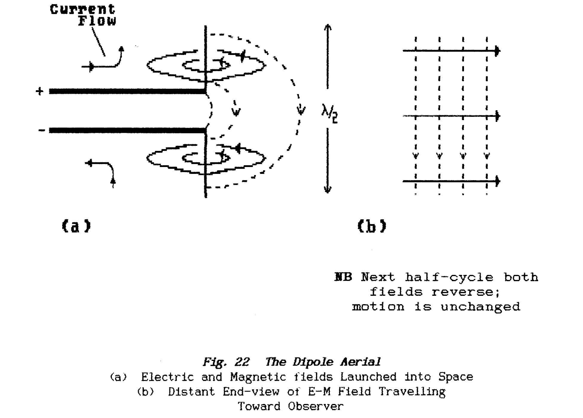
As shown in Fig.22 to obtain maximum leakage from the line requires that the magnetic field be tilted through 900. However the end of an open-circuited transmission line is a point of minimum current-f low (see under 2.3.3); if maximum current is to flow in this aerial the arrangement must ensure that the fan-out includes a point where the current has a maximum value and, for each limb, this is a quarter-wavelength from the very end of the line.
>>>>>>>>>>>>>>>>>>>> PAGE 52 <<<<<<<<<<<<<<<<<<<<
The radiating section which results is an Aerial (antenna in American and Amateur circles) and measures a half-wavelength overall; because it has two (opposing) electric poles it is known as a Dipole or Doublet.
Wavelength is given the symbol λ (greek lambda) and a half-wave aerial is referred to as a λ/2 radiator (spoken as "lamda-by-two" or more simply as "lambda-two" or even as "half-lambda"). Similarly a quarter-wave section is designated as a λ/4 or "lambda-four" section.
Detailed aerial theory is given in many textbooks but the following points are worth noting here:
(a) current cannot flow at the ends of the aerial and so a standing-wave pattern is to be expected on the two "limbs" of the dipole; however, if a match is being achieved between the dipole and the transmission line, then this standing-wave pattern will not extend back along the line (or Feeder) beyond the start of the fan-out
(b) Signal current flows on the feeder in push-pull; i.e. at any given instant current flows from one leg of the feeder into the aerial but from the aerial into the other leg. As shown in the diagram the current in all parts of the aerial flows in the same direction. (This is not true of all aerials,)
(c) The quadrature (900) relation between voltage and current on the aerial seems to be in conflict with the statement above that, in an e-m radiation, the electric and magnetic vectors are always in phase. In fact Maxwell's equations indicate that an e-m field, as it immediately surrounds an aerial, has two components:
(i) an induction field in which the electric and magnetic vectors are in quadrature but which extends only a few wavelengths from the aerial. This field has considerable magnitude and is the cause of short-range interference.
(ii) a radiation field in which the electric and magnetic vectors are in phase and which is capable of extending to great distances.
(Note that the concept of two fields is but an interpretation of mathematics; in practice the field changes from near-quadrature to being in-phase over a few wavelengths as it departs from the vicinity of the aerial.)
** The impedance which a dipole presents at its centre where the feeder is connected is usually in the range 50 to 100 ohms. The exact value depends on the details of the design.
** It is shown in Fig.22 that the current flows in the same direction throughout the length of the dipole; it flows into one leg of the feeder but out of the other. Assuming that the feeder is properly balanced the currents in each leg are equal and so the currents on each limb at the centre of the aerial must be equal. It follows that it does not greatly affect the operation of the device if the two limbs of the aerial are constructed from a single conductor as shown in Fig.23(a).
** It may look like a short-circuit but the standing-wave decrees that the short length of wire at the centre of the dipole has a p.d. across it and that it carries current at the maximum value.
>>>>>>>>>>>>>>>>>>>> PAGE 53 <<<<<<<<<<<<<<<<<<<<
There is a range of possibilities for making the connection between feeder and dipole of which the two extremes are:
(a) feeder connected to the outer extremities of the dipole which effectively terminates the feeder in an open-circuit
(b) feeder connections both taken to the centre of the dipole which terminates the feeder in a short-circuit.
|
** Between these two extremes any desired impedance can be obtained as a termination for the feeder; as shown in Fig.23(b) the end of the feeder is physically fanned-out to be attached at the appropriate points. 2.4.5 The End-fed Dipole The simple introduction above to the simplest of the aerials resulted in a dipole which had the feeder connected at its centre. Because of the low-voltage high-current conditions at the feedpoint this centre-fed dipole is often said to be current fed. ** The basic parameter of the Dipole is that it has two poles or two limbs; these are driven against each other and the most often-used form is a half-wavelength overall at the required frequency of radiation. ** If not too far off frequency a dipole will still radiate well but its centre-point impedance will not be resistive and so a standing-wave will appear on the feeder. In turn this means that the feeder will not deliver to the dipole the maximum possible power. It has been shown already that a dipole need not necessarily be broken in the middle; where it consists of a single length of wire it is possible to drive it at either end instead of at the centre. If this appears to be wrong or somewhat implausible you are to be congratulated; Question: How can power be fed to an aerial through a point where current does not flow? |
** The answer is that we cheat. Each half of a centre-fed dipole is driven against the other; that means that limb-a is first driven positive with respect to limb-b and then, during the next half-cycle, limb-a is driven negative with respect to limb-b. The voltage of each limb is measured with respect to the other (their relative voltage); the absolute voltage (with respect to Earth) is not important as far as driving the dipole is concerned.
** To end-feed a dipole one end only is driven first positive and then negative with respect to Earth. The aerial DOES radiate power as a consequence and so it>>>>>>>>>>>>>>>>>>>> PAGE 54 < < < <<<<<<<<<<<<<<<<<
must be accepted that current flows of necessity from the feeder into the end of the dipole. At the far end of the dipole it is still true to say that current has nowhere to flow and so this is a point of maximum voltage and zero current but, at the driven end (the input end), conditions are not the same.
The dipole supports a standing wave and so the two ends, a half-wavelength apart, could be expected to have similar conditions; they differ by a small amount because the driven end has been modified by connecting a feeder to it. Thus, while the free end is theoretically an open-circuit, the driven end must settle for no more than a high impedance; i.e. it is a point of high voltage and low current rather than zero current.
** The basic difference between the two dipole configurations
therefore is that the centre-fed one requires a low-impedance drive (a current
drive) and the end-fed requires a high-impedance drive (a voltage
drive).
.
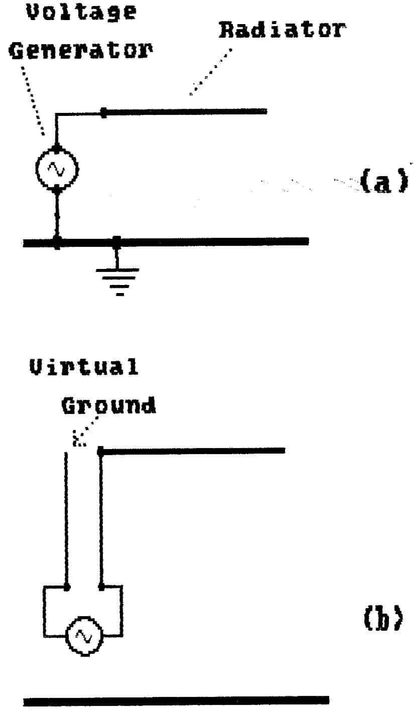 |
. | But how is it achieved? Fig.24 (a) shows the basis of the various systems that have been devised wherein a generator is connected between one end of the aerial and ground. This indeed provides all that is necessary but, to implement this arrangement with practical hardware, would require either a very-large generator or a very-low aerial. Clearly a transmission line must be introduced and it is in this matter that confusion usually arises. ** When a transmission line is taken to the end of a dipole one of its terminals has to be connected to the end of the radiating conductor and the other terminal to ground (against which the dipole is to be driven). The problem of course is that the dipole needs to be elevated above the ground. ** The solution is to provide some kind of artificial ground; a practical stand-in for the ground but which is in fact well above the real ground. A great variety of arrangements have been devised but the most-often seen end-fed dipole just leaves the other feeder connection up there next to the aerial without it being connected to anything. ** Yes, it is unhygienic and yes the practice does incur penalties. The arrangement, as illustrated in Fig.24 (b), is known as a Zepp (or Zeppelin) feed and it can give good results. |
>>>>>>>>>>>>>>>>>>>> PAGE 55 <<<<<<<<<<<<<<<<<<<<
** Six paragraphs above it was said that the feeder modifies the conditions on the aerial at the driven end. It is equally true to say that the feeder-conditions are modified when an aerial is connected to it. By drawing current from one leg of the feeder only, the aerial upsets the relation between the standing-wave patterns of the two legs. Which perhaps is a long-winded way of saying that the end-fed dipole produces an unbalanced mismatch at the feeder-connection.
** On a properly-balanced feeder, whether or not it is connected to a matching load, the current at any given point flows in opposite directions on the two legs. Thus, external to the feeder, little if any field is encountered because the contributions from each leg cancel. When that balance is upset, as it is with a simple end-feed, this cancellation fails and an external field appears around the feeder. In other words the feeder adds its own quota to the overall radiated e-m field. This may or may not be harmful or desirable and it may cause interference.
** The various developments of the end-feed system all aim to correct this imbalance and so prevent radiation from the feeder; they are described in later Sections which deal with aerial-matching. It might be thought that the Coaxial Feeder, which is described in Section 2.3.5, would overcome this difficulty but it is found that, when aerial and feeder are improperly matched, current flows on the outside of a coaxial feeder and so causes unintentional radiation.
END OF LESSON 9
* * * * * * * * * * * *
QUESTIONS
1. How is power carried by a transmission line ? What is the basic principle employed in transforming this power into an e-m wave.
2. An aerial can be viewed as an impedance-matching device which couples a feeder to free space. Standard feeders come in 50-ohm and 75-ohm types; how can both these be matched by a single dipole aerial?
3. Your "shack" of the future might be equipped with both a centre-fed dipole and an end-fed dipole. How would you expect the feed arrangements to differ?
4. In broad terms only would you expect to find a series-resonant circuit or a parallel-resonant circuit driving an end-fed dipole?
5. A network of resistors consists of 20-ohms in series with 10-ohms shunted overall with 30-ohms. A 9-volt battery, connected across the combination, has a measured internal resistance of 3-ohms. What is the terminal voltage of the battery when the network is connected?
>>>>>>>>>>>>>>>>>>>> PAGE 56 <<<<<<<<<<<<<<<<<<<<
In the previous Section it was argued that current flowed on a radiating conductor as a result of its being driven from the end of an energised feeder. However, it cannot be supposed that the radiator "knows" how the current came into being and so it follows that, as long as an alternating current is induced to flow, then the conductor will launch an e-m wave.
Such a current can be induced by placing a conductor in a radiated e-m field. The simplest to understand, and the most effective combination, is when the conductor is a half-wavelength in length and matches the radiator which launched the e-m wave; it also matches the physical dimensions - in terms of wavelength of the wave. The electric component of the field produces a voltage between the two ends of the conductor and so current flows.
The argument thus comes full-circle in that the new conductor with its induced alternating current must in its turn radiate an e-m wave. The phenomenon whereby a conductor first absorbs power from a passing wave and then radiates that power back into space is known as re-radiation. A conductor which is behaving in this manner is referred to as a parasitic radiator - one which is stealing its power.
Parasitic radiators can be very useful devices and are frequently used in constructing aerial arrays in which the purpose is to control the direction in which radiation takes place. (See later under 2.4.9.) It is important to remember however that any piece of conducting material behaves in this manner and, when close to a transmitting aerial, rusty joints or intermittent contacts are responsible for interference (see under E.M.C.) and noisy reception.
The simple development of the dipole aerial appears in Fig.22 to refer to a vertical aerial but in fact the argument is not altered by turning the dipole/feeder assembly through 90-degrees thus forming a horizontal dipole. When considered as a radiating element in free space the terms vertical and horizontal are meaningless.
While the attitude of any particular conductor is not important to launching an e-m wave it matters a great deal when trying to recover the wave by absorbing it into another conductor. The electric component of an e-m field will not induce an emf into a parasitic conductor unless that conductor is aligned with the electric component.
The direction of the electric component is known as the polarisation of the radiated wave and clearly it is defined by the radiating conductor. Thus a horizontal dipole is said to radiate a horizontally-polarised wave and a vertical dipole radiates a vertically-polarised wave.
The use of a dipole in the wrong attitude does not necessarily preclude the establishment of a communication channel but it very much weakens the received signal. Cross-polarised working is possible because the plane of polarisation is disturbed by re-radiation and also during propagation (see later).
>>>>>>>>>>>>>>>>>>>> PAGE 57 <<<<<<<<<<<<<<<<<<<<
A practical point (which is not very important for the R.A.E.) is that a horizontal dipole is balanced with respect to Earth while a vertical dipole has its lower limb closer to Earth and so is subject to increased stray capacitance on that limb. Unless the vertical dipole is mounted several wavelengths above the Earth's surface an out-of-balance current flows on the outside of a coaxial feeder and causes difficulty with matching.
Most practical aerials are required to operate within a few wavelengths of the Earth's surface (or some other surface such as the skin of an aeroplane). Any part of the e-m field which is radiated below the horizon line causes rf currents to flow in the adjacent surface which therefore acts as a parasitic radiator and re-radiates a secondary signal.
As illustrated in Fig.25 this re-radiated signal can be regarded as a reflected signal and so the surface acts as a mirror. The re-radiated signal appears to come from a secondary aerial below the surface.
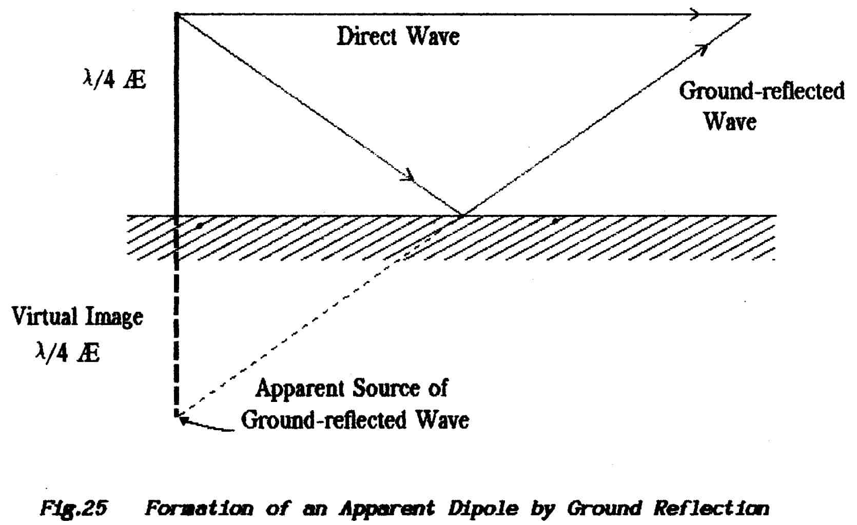
This is an extremely useful phenomenon where long wavelengths mean that a λ/2 dipole will be physically too large for a practical construction; the conductor is cut to a length λ/4 and mounted over a reflecting (re-radiating) surface so that it appears effectively to be λ/2. The resulting half-dipole has only a single "pole" and so it is often referred to as a unipole. Very often the supporting mast becomes the vertical aerial; where the mast lacks the height to resonate at λ/4 it is loaded with a coil (in effect the extra height required is coiled up) and such a device is known as a Marconi Aerial.
>>>>>>>>>>>>>>>>>>>> PAGE 58 <<<<<<<<<<<<<<<<<<<<
The unipole aerial is useful at high frequencies in solving the problem of providing a virtual earth; the quarter-wave radiator is mounted above a reflecting surface which is connected to the external shield of a coaxial feeder.
The reflecting surface is known as a counterpoise or as a ground plane and it should be at least λ/4 in radius. A difficulty with such a ground plane is that it offers considerable wind resistance and so the reflecting surface may be replaced with a wire mesh or by a system of λ/4 rods. Such rods are usually four in number radiating at 900 intervals; occasionally aerials are seen with only two such rods but, in practice, it is found that their number and direction is of less importance after the first one has been connected.
A unipole is essentially one-half of a centre-fed dipole and so its driving-point impedance (dipole-end to groundplane) is around 35 ohms.
A directional aerial is one which radiates the majority of its power in a given direction. However the same aerial when used for reception concentrates its receiving performance in that same direction. Such aerials can therefore provide a gain with respect to a simple dipole; note however that they do not amplify the signal but merely concentrate in one direction the power that otherwise would be broadcast. The gain is available at both ends of a communications channel.
Directivity results from radiating two (or more) signals from points which are separated by a critical distance; the separation means that in some directions the two signals are in phase and so add to form a large signal while, in other directions, the two signals are out-of-phase and mutually cancel. This is illustrated in Fig. 26.
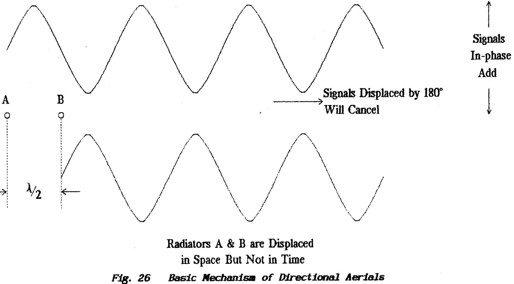
>>>>>>>>>>>>>>>>>>>> PAGE 59 <<<<<<<<<<<<<<<<<<<<
The two positions A and B represent two radiators which are separated by a half-wavelength but which are fed with identical signals . The overall field which they lay-down depends on the position of the reception point; along their common line either in direction AB or BA one signal arrives a half-cycle later than the other and so cancellation results; at 900 to the common line the signals arrive simultaneously and so add.
As an alternative the two radiators could be fed with signals that are 180 out of phase; in such circumstances the maximum radiation occurs along the line AB and minimum radiation at 900 to the common line.
The interfering signals are derived either by sharing the available power between separate radiators or by making one radiator parasitic on the other. The first technique results in so-called arrays; the various forms of curtain array, end-fire array, broadside array, steerable array etc. are described in the literature. Such aerial systems require a lot of room with substantial masting and rigging and are not of interest in Amateur circles.
The second technique using parasitic elements comes into its own at those frequencies where the wavelength makes it practical to use self-supporting rods as the radiators. The ultimate in such designs is the greatly-favoured Yagi aerial.
The first step is to place a parasitic element (or a reflecting plate/mesh) "behind" the radiator to act as a reflector. The resulting "H" aerial was a common domestic feature during the reign of the Band-I Television Service. The reflector and radiator both are resonant (or tuned) elements and so their length is critical; if cut over or under the correct length their impedance exhibits either inductance or capacitance which causes phase-shift effects. Such phase-errors can be corrected by altering the spacing of the two conductors and this facility is exploited to design aerials which are smaller than the basic λ/2 dipole
The next step is to add other parasitic resonators (directors) "in front of" the driven radiator; there is little point in placing them behind the reflector. These are usually cut progressively shorter toward the front of the aerial and again correction is applied by varying the spacing. Not only does such trickery reduce the physical size of the aerial but it allows the bandwidth and matching to be adjusted.
Bandwidth as applied to an aerial is the range over which its driving-point impedance matches a given feeder but, in practice, it is very much a matter of how it is defined. A yagi aerial is essentially a set of resonators coupled together electromagnetically. Coupling means that an adjustment to any one radiator causes a change in the impedance coupled into all the others and so they become detuned. As a result it is all but impossible to set-up such an aerial with accuracy so that it gives a constant performance over a required range of frequencies.
The best that can be required is that it should remain within a certain swr but even that proves to be difficult except at a few spaced frequencies, This is why television aerials are specific to areas and there is seldom any point in taking the aerial with you when you move house.
The above description shows that power is concentrated in a given direction but is does not make clear that this effect takes place both around the horizon (in azimuth) and also in the vertical plane (in altitude). Thus a multi-element yagi is
>>>>>>>>>>>>>>>>>>>> PAGE 60 <<<<<<<<<<<<<<<<<<<<
capable of producing a pencil-like beam which has some very distinct disadvantages. Such an aerial must be aimed very accurately in both azimuth and altitude or it may cause signal-attenuation instead of the intended signal-gain.
To complicate matters still further the addition and cancellation of signals is seldom that complete and the pencil beam is found to be accompanied by a whole family of side lobes; some of these side-lobes may be in the rearward direction where the reflector is supposed to have eliminated radiation. The gaps between lobes (null points) are usually fairly sharply defined and can be useful in eliminating powerful interfering signals during reception but it is all too easy to align a yagi aerial so that one of the side-lobes is in operation rather than the main lobe.
There are two important parameters of directional aerials about which there is often confusion:
(a) Front-to-back Ratio This is the ratio of signal strength radiated (or received) in the forward direction to that radiated in the rearward direction. (For those aerials in which a rearward lobe does not exist then the nearest side-lobe is used,)
(b) Aerial Gain This is the actual forward gain which the aerial affords relative to a simple dipole because it diverts all the power into a given direction. (Strictly speaking it is measured with respect to a theoretical perfect radiator, known as an isotropic radiator, which radiates equally in all directions throughout a sphere; in practice it is generally of more interest to compare with a simple dipole.)
The difference is easiest to grasp by considering that an inefficient aerial may have a large back-to-front ratio (i.e. may be very directional) yet produce a signal which is poor in comparison with that from a dipole.
In multi-element aerials such as the yagi described above each parasitic element absorbs power from, and therefore loads, the driven element. The effect of this is to lower the driving-point impedance of the main radiator and so make it difficult to achieve an impedance-match to the feeder.
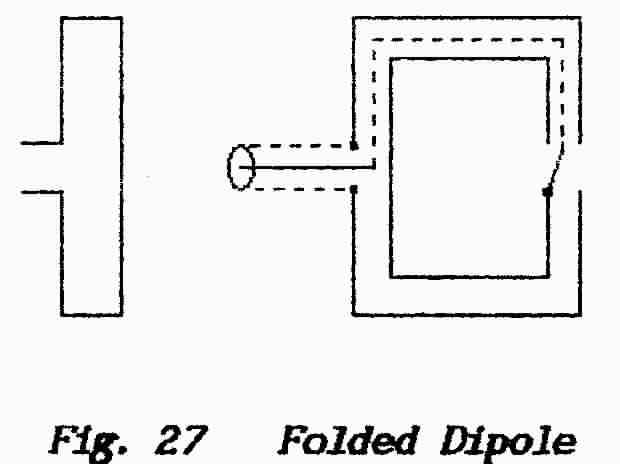 |
The folded dipole illustrated in Fig.27 can be regarded as a "squashed" loop and, as with the Loop Aerial described in the following Section, it offers a driving-point impedance of 300 ohms. This is of course reduced by the proximity of parasitic elements but the final value is closer to the 50-ohms or 75-ohms of standard coaxial feeders. |
>>>>>>>>>>>>>>>>>>>> PAGE 61 <<<<<<<<<<<<<<<<<<<<
This aerial is often referred to (mistakenly) as a magnetic loop. To achieve communication over any distance an aerial must generate e-m waves. The magnetic or induction loop is used at low (even audio) frequencies and is characterised by its very limited range outside the area of the loop.
The impedance presented by a radiating loop is around 300 ohms and it does not support a standing wave.
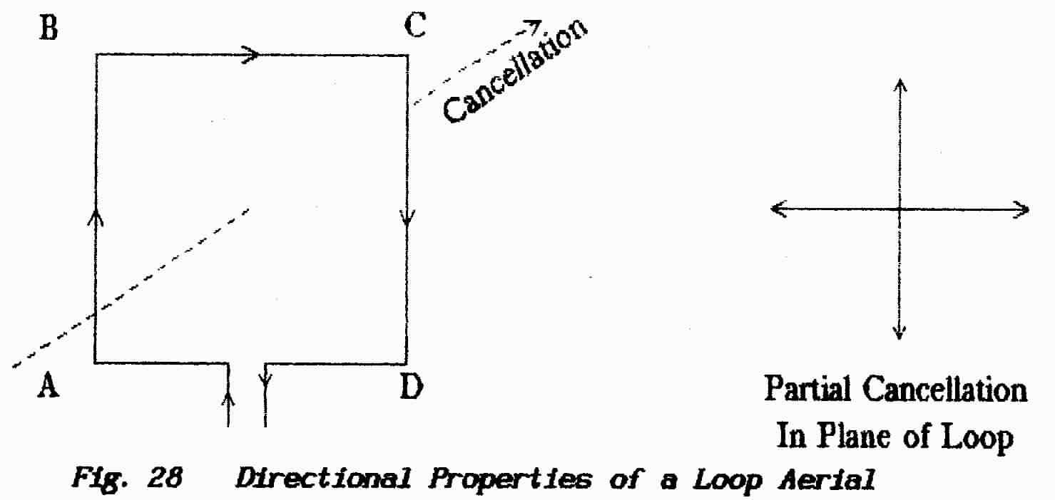
Because the loop-current is uniform (i.e. a standing-wave is not present) the external field is the direct sum of the e-rn field radiated by the opposing limbs. In Fig.28 the current in AB opposes that in CD when viewed from a point on the loop's axis and so cancellation takes place in this direction. When viewed from any direction in the plane of the loop such cancellation cannot be total because of the phase difference produced by the different distances from the observer.
Thus a loop aerial shows directional properties but it cannot be classed as a beam aerial because it is not diverting power into any given direction and is not providing a gain.
The radiation pattern of a loop is a single lobe which resembles a large doughnut surrounding the loop. When mounted vertically a loop provides a sharp null in azimuth; this can be useful in reception for eliminating an unwanted signal and is also used for direction finding. For transmitting purposes however a loop is best used horizontally in which position it covers 3600 in azimuth and most of the useful angles in altitude (see later Skywave under Propagation).
An interesting property of loop aerials is their ability to work at any height above ground from zero upward. They also pick-up very little background noise.
>>>>>>>>>>>>>>>>>>>> PAGE 62 <<<<<<<<<<<<<<<<<<<<
Aerials for both transmitting and receiving (or both) are available in a multiplicity of forms which are well documented in the literature. Their study here would not add anything to the general understanding of the subject and this Course does not deal further with them. However I am always willing to accept questions or requests for help.
END OF LESSON 10
* * * * * * * * * * * *
QUESTIONS
1. What is the purpose of a parasitic radiator?
2. What is meant when a radiation is said to be vertically polarised?
3. What is the essential component of a unipole aerial?
4. Why is it that a loop aerial cannot be regarded as a beam aerial?
5. Why is a folded dipole commonly seen in multi-element aerial arrays?
6. A circuit used to couple a transmitter to a feeder consists of a series inductor followed by a capacitor connected to Earth. In terms of frequency only how would you expect such a circuit to behave?
7. A tuned parallel-circuit with a measured Q of 20 draws 20 mA from a generator by which it is being driven at its resonance frequency. What is the circulating current within this tuned circuit?
>>>>>>>>>>>>>>>>>>>> PAGE 62 again <<<<<<<<<<<<<<<<<<<<
The term propagation refers to the manner in which radio signals travel from a radiating aerial to a receiving site. The behaviour of a propagating e-m wave depends on its frequency (or wavelength), the time of day, the time of year, the nature of the Earth's surface-covering, the condition of the Earth's atmosphere and on the sunspot cycle.
In Lesson 9 it was stated that a transmitting aerial sets-up a radiation field that can be regarded as two separate components namely an induction field and a radiation field. The induction field does not extend beyond a few wavelengths from the aerial.
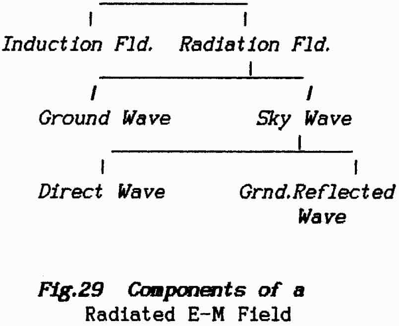 |
The radiation field can itself
be divided Into two separate components as shown in Fig. 29. One
of these is dependent on currents which flow in the Earth's surface
and so it remains close to the ground and is known as the ground
wave The launch of such a wave is possible
only by a vertical aerial which is at a height comparable with the wavelength.
(The electric component of any ground wave launched by a horizontal aerial
would be short-circuited by the Earth.)
The propagation of a ground-wave depends on the conductivity of the earth and its energy is dissipated in earth currents. Ground-losses increase with frequency and so range decreases as frequency rises. |
The other component, independent of the Earth, is known as the space (or sky) wave. This component is itself divided into a direct wave and a ground-reflected wave. The Earth's upper atmosphere is powerfully irradiated by the Sun and this causes it to ionise; i.e. to break up into positively-charged and negatively-charged particles (ions) which are capable of carrying electric currents. These form in several layers at different heights and, by absorbing and re-radiating rf energy, they act as "reflecting" layers. The Sun's activity varies in an 11-year cycle and this is reflected in the number of sunspots visible on its disc. Thus sky-wave propagation phenomena are linked to the Sunspot Number.
In general signals which are radiated at high angles of elevation tend to pass straight through these layers and are lost to Space. Radiation below certain critical angles is returned to Earth with varying effects. The distance between the transmitting site and the point where the signal returns to Earth is known as the skip distance.
At frequencies up to about 300 kHz the ground wave is very strong, propagates over very-long distances and may penetrate to a significant depth; frequencies around 15 to 20 kHz are used to communicate with submerged submarines.
>>>>>>>>>>>>>>>>>>>> PAGE 63 <<<<<<<<<<<<<<<<<<<<
In the frequency range 20-kH to 100-kHz both ground-wave and sky-wave absorption is very low and most of the transmitted energy can reach receiving points up to 1,000 km by way of the ground wave. Received signals show very little daily, seasonal or yearly variation.At very great distances where the ground-wave is completely absorbed the received signals are entirely sky-wave and show diurnal (day & night) and seasonal variations; the strongest signals occur at night and in the Winter. Transmission is also characterised by a sudden drop in signal strength when the sunset line falls across the transmission path but, otherwise, fading does not occur at these very low frequencies.
In the frequency range 100-kHz to 550-kHz the ground-wave attenuation increases thus raising dependence on the sky-wave for distance communication. Sky-wave attenuation however tends to be much greater in the daytime and in the summer and, in general, long distance communication at these frequencies is not possible during the day particularly in summer.
This Band extends from 300 kHz to 3 MHz ( λ/4 = 250 to 25 metres) and quarter-wave resonant conductors become practicable; at the lower end of the Band the Marconi-type λ/4 vertical radiators are typical. The ground wave is less extensive but extends over sufficient distance to permit domestic broadcast services. For this purpose the signal needs to be of sufficient strength to override interference and be as free as possible from fading and distortions. The area where such conditions prevail is known as the primary service area which typically extends to around 50 - 100 miles.
Reflection at the lowest of the ionised layers (the D layer) gives the shortest distance between transmitter and the return point but, because sky-waves at broadcast frequencies are completely absorbed in the daytime, broadcast signals rely entirely on ground-wave propagation.
After dark, as the ionisation decreases, the D layer disappears and signals are reflected from the E layer above it (and sometimes by the F-layer also). Close to the transmitter the reflected sky-wave is weak and so the ground-wave predominates. As the distance from the transmitter is increased so the ground-wave becomes attenuated but the sky-wave increases in strength and so the primary service area becomes surrounded by one in which the two signals are of similar strength.
The reflecting layers are not rigidly bounded and so the effective height from which reflection takes place is variable; this means that the relative phase between ground and sky waves is constantly changing and so the two signals vary between mutually aiding and mutually canceling. The result is the after-dark fading which is familiar to all who listen to medium-wave broadcasts at some distance from a transmitter.
Another feature of this area is selective fading. Whether ground-wave and sky-wave cancel or aid is determined by the difference in path lengths as measured in wavelengths. The wavelength differs for each side-frequency and so the relation between carrier and sidebands is greatly disturbed. This results in severe distortion which varies in much the same way as does fading.
Beyond the effective area of the ground-wave the sky-wave remains useful for long-distance communication but with limitations.
>>>>>>>>>>>>>>>>>>>> PAGE 64 <<<<<<<<<<<<<<<<<<<<
Signals sometimes propagate over more than one path between transmitting and receiving aerials which means that fading and distortion can occur even in areas where the ground-wave does not exist. These effects occur to a much lesser extent that when a ground-wave is present.
Ground-wave signals in the Long and Medium Wavebands decrease in direct proportion to the distance.
The short-wave Band, which ranges from 3 MHz to 30 MHz, includes all the hf bands permitted for Amateur use except the so-called Top Band (1.8 to 2.0 MHz). At these frequencies the ground wave is rapidly dissipated and does not offer any real facilities. Amateur operating is permitted only in specified ranges of which the higher-frequency bands are of real use only during periods around sunspot maxima.
In this Band a quarter-wave is between 25 & 2.5 metres and so efficient aerials can be built in many forms including multi-element directional units.
Aerials may be erected either vertically or horizontally but it is not practical for the Amateur to set them very far (in terms of wavelengths) above the Earth's surface. Their radiation must therefore set-up ground currents and so ground conductivity plays an important part in performance. Over-sea paths perform best but it is common practice to use one or more ground-wires or counterpoises to improve conductivity at the launch site.
Between the outer edge of the ground wave and the point where a sky-wave returns to Earth there is an area where signals cannot be received. At the return point however a signal with sufficient strength can set-up earth currents and so be re-radiated (or re-reflected); such re-radiation follows the optic rule that the angle of reflection is equal to the angle of incidence and so the sky-wave is re-launched toward the Ionosphere to be reflected once again. Thus a series of skips (or hops) make it possible to communicate beyond the horizon and indeed all around the globe.
However things are seldom perfect and this world-wide progress makes its own demands. To communicate by sky-wave it is necessary to ensure that the target area does not lie within one of the skip zones. This requires that the sky-wave be launched at a certain angle and it must suffer reflection as against passing straight through the reflecting layers. To ensure reflection means choosing a frequency that will be reflected by the appropriate layer at the given time of day and at the given angle of incidence on that layer.
Needless to say the prediction of "correct" frequencies is a science in its own right and the work is based on daily measurements. These predictions are published in table form for the benefit of the communications world; one source for the Amateur is the monthly publication of the Radio Society of Great Britain Radio Communication or RadCom. Most amateur aerials radiate over a fairly-large range of elevations and so the only requirement is to use the correct frequency-band for the chosen destination and time of day.
Depending on the frequency and angle of launch a reflection of the sky-wave may take place at any of the ionospheric layers and so several different paths may be available. Over long-distance routes propagation differs markedly between east-west paths and north-south paths. This is because of the different distributions of sunlight and different seasonal variations along those paths.
>>>>>>>>>>>>>>>>>>>> PAGE 65 <<<<<<<<<<<<<<<<<<<<
There is benefit to be obtained from using aerials with directional properties both in azimuth and elevation. Reflection from the Ionosphere is best when the propagating wave enters at low angles but, if the wave is too close to the horizontal, it is absorbed by the ground. Vertical λ/4-type aerials are often used because they give good low-angle radiation.
Vertically-polarised and horizontally-polarised aerials are equally successful for transmitting because, on reflection from the Ionosphere, signals are found to possess both vertically-polarised and horizontally-polarised components which bear no apparent relation to the polarisation of the transmitting aerial. These two components fade independently and are not in phase. These effects are mainly caused by the Earth's magnetic field.
Communication channels in this band are sometimes completely cut for periods of 15 to 60 minutes by what are known as sudden ionospheric disturbances or S.I.D's. This is believed to be caused by absorption in the D-layer caused by bursts of ultraviolet light from the Sun.
The VHF Band (very-high frequencies) extends from 30 MHz to 300 MHz and the UHF Band (ultra-high frequencies) from 300 MHz to 3,000 MHz. At these frequencies the ground wave is non-existent; usually the aerials are mounted several wavelengths above the Earth's surface and consist either of balanced dipole-types or ground-plane quarter-wave types.
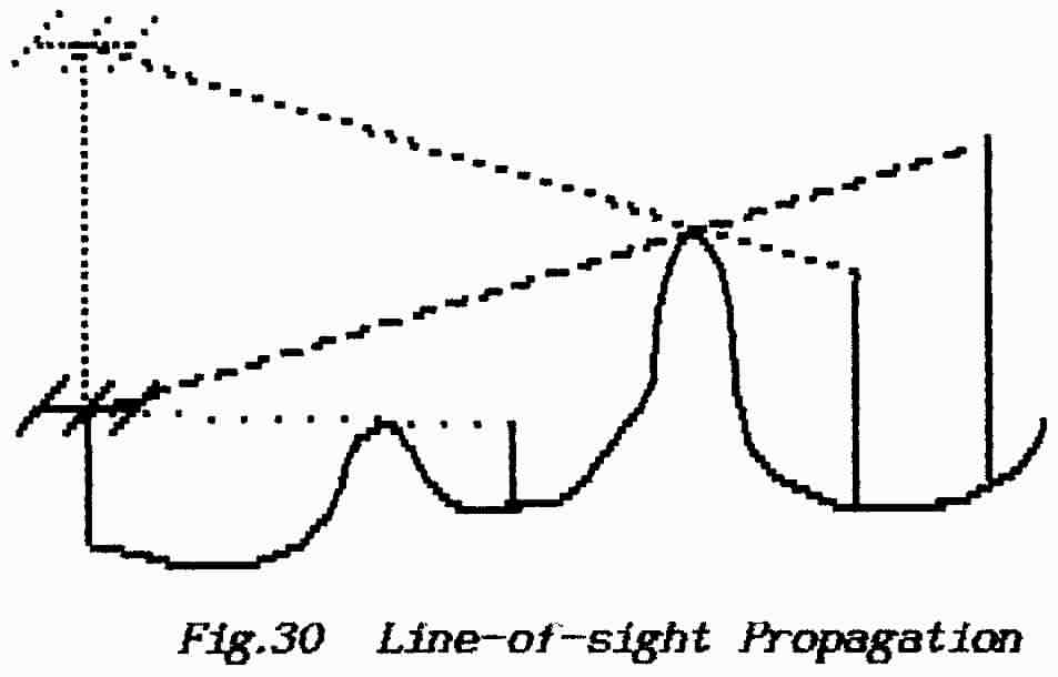 |
At these frequencies skyward radiations pass straight through the ionised layers and so all that is left is the direct-wave which propagates along the line-of-sight path. As shown in Fig.30 the distance over which communication can be achieved is governed by the height of both the transmitting and receiving aerials. The diagram shows a true geometric construction but, in fact, the path-length is greater than indicated. This is because the e-m wave tends to be refracted by the Atmosphere and follows a curved path which effectively lowers the intervening horizon. A reasonable prediction of path length can be made by assuming that the Earth's radius is 4/3 its true radius; i.e. approx 5,200 miles. |
It follows that the range over which communication can be achieved at vhf and uhf is dependent on the height of the transmitting and receiving aerials.
This distance can be drastically shortened however where a tall building or a hill breaks the transmission path. Although structures such as these are opaque to very-high frequencies weak signals can be obtained in their radio-shadow due to a phenomenon known as diffraction. Because of interference effects at an edge a portion of the field is bent down into the shadow area. Additionally the signal may arrive in the shadow region by reflection from objects on other bearings so effectively directing a signal around the obstruction. In television-engineering such multipath propagation causes echoes known as "ghosting".
>>>>>>>>>>>>>>>>>>>> PAGE 66 <<<<<<<<<<<<<<<<<<<<
An elevated vhf or uhf aerial launches a signal directly toward or over any receiving aerial but it is not prevented from radiating below the direct line-of-sight path. Such signals must strike the Earth's surface, they induce current-flow and so suffer reflection. As shown in Fig.31 this reflected signal travels over a longer path than the direct signal; the path difference (in wavelengths) will depend on the overall separation of transmitting and receiving aerials, on the height of each above the ground and on the frequency.
|
On reflection at these low angles the signal suffers a phase-change of 1800 with the result that the direct and reflected waves tend to cancel and so reduce the strength of the received signal. As one or other of the aerials is raised so there must be a steady increase in the path difference, the cancellation is reduced and the received signal increases in strength. This phenomenon is referred to as height-gain. |
Although there is a real bonus available by mounting vhf and uhf aerials as high as possible (apart from line-of-sight considerations and avoiding the screening action of buildings etc.) the height-gain effect does not continue endlessly. At some point the path difference reaches 1800 and further increase in height will result in a height-loss. This is a consideration only in commercial fields where masts of 500-ft or more may be worth considering but the planners need to be aware that the additional cost of a higher mast might result in a signal loss. Height-gain is taken for granted in Amateur circles although a few who live on the edge of high ground may find that their ground-reflection point is on a plain several hundred feet lower and could result in a height-loss.
Where propagation involves interaction between direct and ground-reflected components of a space-wave the signal is attenuated inversely as the square of the distance; compare this with the attenuation of a
Anomalous Propagation
This term is applied to signals which arrive unexpectedly and apparently by breaking the accepted rules. It is usually the result of the signal encountering a propagation path wherein the attenuation is less than normal.
Apart from the regular ionised layers there is an irregular and unpredictable type of ionisation which occurs at about the level of the E-layer. This takes the form of "clouds" which may be many kilometres across and which may last from a few minutes to a few hours. These clouds have been known to reflect signals up to 80 MHz and such propagation is known as sporadic-E. Sporadic-E does not occur when weather systems keep the Atmosphere well mixed.
>>>>>>>>>>>>>>>>>>>> PAGE 67 <<<<<<<<<<<<<<<<<<<<
In general the properties of the Atmosphere follow a standard pattern with height above the Earth's surface but irregularities in temperature-gradients and moisture content often bring about changes in the manner in which the Atmosphere refracts (bends) e-m waves. Instead of producing the effect already mentioned whereby the Earth can be considered as having its radius increased by 4/3 the refraction may be either increased or decreased.
Abnormal refraction can result in the path of a propagating wave following the Earth's curvature thus traveling distances much greater than normal. At high frequencies it is possible for the wave to be trapped between two layers thus drastically reducing attenuation. Such effects are known as ducting.
The path can also be bent away from the Earth's surface so reducing the range.
Other areas of ionisation produce visual effects
known as the Aurora and these too can be used for communicating over paths
not otherwise available. Yet another path often explored by Amateurs is to "bounce" signals
off the surface of the Moon.
END OF LESSON 11
* * * * * * * * * * * *
QUESTIONS
1. What are the causes of fading?
2. Above 30 MHz what determines the maximum range of reliable transmission?
3. Why is it that in the Amateur Bands we can use either vertically-polarised or horizontally-polarised aerials as convenient?
4. What is the difference between a counterpoise as it might be used under an amateur short-wave aerial, and a ground-plane?
5. Why is the choice of frequency important to establishing radio contact on short-waves?
6. Why are vertical λ/4—-type aerials useful in long-distance contacts?
7. Why do tall buildings or other radio-opaque features disrupt communications at vhf but not on short-wave bands?
>>>>>>>>>>>>>>>>>>>> PAGE 68 <<<<<<<<<<<<<<<<<<<<
** A receiver has 10 basic requirements:
1. To accept from an aerial/feeder system the energy which has been extracted from passing e-m waves and select from the mass of signals the one that is required.
2. To maximise the wanted signal and to reject as much as possible the remaining signals and extraneous noise.
3. To add to the required signal as little noise of its own creation as possible.
4. To amplify that signal to a level at which it can be processed without degradation.
5. To extract from the signal the information which it carries as some form of modulation.
6. To amplify the information signal to a specified power level so that it may drive the requisite termination gear: e.g. loudspeaker, printer, servo-motor.
7. To provide automatic and/or manual control of signal levels at all stages of the receiver.
8. To remain "tuned" to the frequency of the required signal without constant attention.
9. Not to cause radiation of signals via the aerial system to which it is connected.
10. To remain unaffected in its operation by powerful signals which may, for example, emanate from nearby transmitting equipment.
** Although a receiver operates as an entire system it can be broken down into a number of distinct units as illustrated in the block diagram of Fig. 32.
(a )**Aerial Attenuator
The input circuits of receivers, and especially those utilising semiconductors, are easily overloaded by strong signals. When this happens the input circuits lose their ability to select a wanted signal — the receiver becomes untunable. This effect can be caused either by the wanted signal or by an unwanted signal against which the selective circuits should discriminate.
The aerial attenuator is usually a set of resistive pads which can be switched-in by the Operator so as to reduce the signal level which reaches the receiver input. In some sophisticated receivers this process is automatically controlled.
(b)**Aeria1-coupling and Tuning Circuits
In this section receivers fall roughly into two categories:
(i) Domestic receivers intended to be used with reasonably-strong signals (that will swamp any ambient noise) and with any kind of aerial including a simple length of wire;
>>>>>>>>>>>>>>>>>>> PAGE 69 <<<<<<<<<<<<<<<<<<<<
in these the input-tuning (selective) circuits also perform the task of matching and tuning the aerial. Mostly such a description is but a euphemism; the best that can be achieved is to "hold off" the aerial so that it does not destroy the performance of the tuned circuits.
** Ferrite—rod aerials, in which a rod of magnetic material is used to concentrate the e-m fields, can largely overcome the problem.
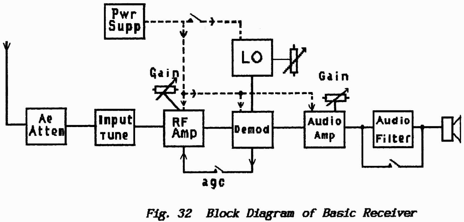
** (ii) Communication Receivers
As the name implies these receivers are used in communication channels and the prime requirement is reliability in performance and the ability to extract weak signals (sensitivity). Thus they are intended for use with properly-engineered aerial systems.
The aerial-tuning circuits therefore are required only to select the required frequency; they are presented with a feeder that requires a resistive termination usually either 75 or 50 ohms.
(c)** Radio-frequency (rf) Amplifier
This part of a receiver, plus the input-tuning circuits, is often referred to as the front end. Its purpose is to raise the selected signal to a higher level where it can be processed without being degraded by the addition of noise.
The rf-amplifier uses tuned circuits in place of resistive loads and so provides further selectivity. Noise generated in the receiver is only significant at the input to the rf amplifier where the incoming signal is at it weakest; it is here that the noise performance of a receiver is established.
To cope with the very-wide range of signals incoming from the aerial the gain of the rf-amp is made adjustable; this control is turned down when receiving strong signals thus suppressing the noise (and weak signals!) heard at the output of the receiver. Usually such gain adjustment is incorporated in an automatic gain-control (a.g.c.) circuit but, in communication receivers, it is not uncommon for an additional manual control to be fitted together with a facility for disconnecting the a.g.c. A.G.C. has a primary function in combating fading.
>>>>>>>>>>>>>>>>>>> PAGE 70 <<<<<<<<<<<<<<<<<<<<
(d) ** Demodulator
In early receivers this section was known as the detector stage and its function is to extract the information content from the incoming signal. Now, with the use of a.m., f.m. and ssb in a single receiver, the more comprehensive term is used. Details are given in later Sections.
The demodulator stage is also used to derive a dc signal whose amplitude is proportional to the signal strength incoming to the demodulator. This is used to operate the a.g.c. circuit; it is a negative-feedback arrangement that tends to maintain the signal level at a constant value at the point of demodulation (i.e. the point at which the agc-control signal was extracted).
For c.w. working (Morse code) a somewhat different method of "demodulation" is required in the form of a local oscillator (L.O.), known as a beat-frequency oscillator (B.F.O.) that can be set to beat with the incoming carrier thus forming an audible signal at the receiver output. The frequency of this audible tone can be adjusted by the Operator through use of a L.O. or BFO control which affords a fine adjustment of audio frequency.
An LO On/off switch must be provided also else this oscillator will render the receiver useless for other types of reception. However, for those receivers not equipped to demodulate ssb signals, it is possible to use the L.O. as a carrier-injection oscillator; this requires considerable skill on the part of the Operator however as, apart from accurate adjustment of the L.O. frequency for either upper or lower sideband as appropriate, it is necessary to achieve correct balance between the levels of ssb and L.O. signals. A manual rf-gain is a great help in such activities and, of course, it is preferable to switch-off the a.g.c.
Reasonable frequency stability is desirable from the L.O. if the output-tone is not to require constant re-adjustment; this is particularly important where narrow-band audio filters are in use to reduce noise. Also to use the L.O. successfully for ssb reception it is essential that it be very stable in frequency.
(e)** Audio Amplifier
The general requirement here is to accept the low-power audio signal delivered by the demodulator and raise it to a power level suitable to drive the final equipment. This might be a loudspeaker, a pair of headphones, a recording milliameter, a servo-system as in model-control or any combination of a variety of purposes.
In domestic receivers the requirement is quality which means a full frequency bandwidth, low distortion levels, low hum and other noise levels and sufficient power to drive a loudspeaker or perhaps more than one loudspeaker.
In communication receivers the requirements are almost the opposite. To reduce noise levels bandwidth is restricted to "telephone quality" - i.e. roughly 300 Hz to 3.5 kHz. For c.w. working the audio bandwidth may be restricted, at the Operator's discretion, to as little as 100 Hz provided that the requisite frequency-stability is available. A certain amount of distortion is acceptable if it is necessary to enable information to be extracted from weak signals.
Output-power requirements are less for a communications receiver. Usually they are fitted with a switched output, suitable to drive a loudspeaker, and one or more outputs to drive headphones.
>>>>>>>>>>>>>>>>>>>>
PAGE 71
<<<<<<<<<<<<<<<<<<<<
** Manual control of audio gain is usual but communications receivers are built in which the a.g.c. is derived from the audio circuits thus ensuring that the audio level remains constant. These receivers also have circuits to restrict the audio bandwidth as already mentioned. Such circuits may be audio filter-networks incorporated in the audio amplifier stages or in the feed to the loudspeaker; alternatively they may be incorporated in the rf-amplifier circuits where they restrict the bandwidth and so eliminate the appropriate side-frequencies.
(f) ** A Power Supplier is necessary where a receiver is to operate from the ac-mains supply (see Part 5 of this Course). Receivers are powered from batteries usually for portable operation but battery-operation is also used where reception/measurement of very-weak signals requires a low noise level. The most common requirement for portability is in equipment intended for mobile use in vehicles; the normal 12-volt battery system is utilised.
Many equipments are fitted with dual mains/battery facilities.
** The simplest of all receivers is the tuned radio-frequency receiver which is restricted to a.m. working. This is a straightforward receiver which follows almost exactly the outline given in the previous Section. The price paid for the simplicity is a lack of selectivity which means that it can be difficult to separate a wanted signal from a nearby powerful signal.
** The TRF receiver does have advantages however. Within the primary service area of a domestic broadcast transmitter (where a strong signal is guaranteed) the lack of selectivity means that a large range of side-frequencies is admitted which provides very good performance in terms of audio bandwidth. The receiver is also immune to the self-generated whistles which are a feature of the more complex circuits described below.
The simplest TRF receiver is the one-valve Leaky-grid Detector (or simply grid-detector). This can be built using a transistor but its operation is easiest to follow in the valve form. It is illustrated in Fig.33.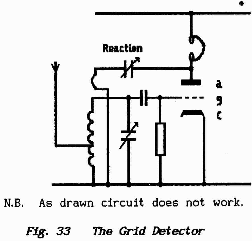 |
A valve responds to the voltage which is impressed between its grid (dotted-line) and cathode. As long as the grid remains negative with respect to the cathode it cannot draw current from the heated cathode. It is usual to add a dc negative bias voltage to any signal to ensure that the positive swings of the signal do not take the grid into conduction. In the grid detector this bias is omitted and so the grid is driven into conduction by the positive swings of the modulated carrier. The grid current charges the grid capacitor and so generates a bias voltage which at all times is proportional to the carrier amplitude. |
>>>>>>>>>>>>>>>>>>> PAGE 72 <<<<<<<<<<<<<<<<<<<<
Finally the current which flows from cathode to anode is determined by the grid voltage. Headphones connected as shown respond to the audio component of the anode current as it varies in sympathy with the varying grid-cathode voltage.
Allowing the grid to conduct reduces the input resistance between grid and cathode and this loads the tuned aerial circuit; in turn this reduces the circuit Q-value and so destroys both its selectivity and its magnification.
The circuit Q can be restored and/or improved by using positive-feedback; the anode current contains a component at the carrier frequency and this is fed back in-phase to reinforce the current which circulates in the aerial tuned circuit. The arrangement, known as regeneration or as reaction makes
Its disadvantages however are serious:
(a) If the Reaction control is advanced too far the p.f.b. becomes excessive and the circuit bursts into self-oscillation at the resonance frequency to which the aerial circuit is tuned. Efficient transfer between aerial and tuned-circuit is a necessary part of the receiver action and so, when oscillation commences, the circuit turns into a transmitter — to the annoyance of everyone who is trying to operate around that frequency. -
(b) The receiver is at its most sensitive just before the onset of oscillation when the circuit Q is at its greatest usable value. However the high Q-value means that the bandwidth is at its narrowest.
(c) It has been shown under 1.13.2, 1.14.3 (Lessons 9+10 in Fundamentals—i) that the Q, impedance and magnification of a tuned circuit vary as the circuit tuning is adjusted. Thus this simple receiver either becomes insensitive or oscillates when any attempt is made to re-adjust the tuning.
** The next logical step in developing the TRF receiver is to isolate the tuned circuit from the aerial so that, should it oscillate, it does not create a nuisance. This requires the addition of an RF Amplifier; this circuit accepts the input from the aerial, selects the required signal, amplifies it and then passes it to the tuned circuit that feeds the grid detector. If properly designed the rf-amp will not pass signals from its anode circuit to its grid circuit and so the aerial is protected (or buffered) from the detector stage.
** To drive a loudspeaker rather than the headphones an audio power-amplifier stage can be added thus producing the 3-stage TRF receiver shown in block form in Flg.34. With such an arrangement it is possible (and permissible) to adjust the detector for a weak oscillation to enable reception of cw signals.
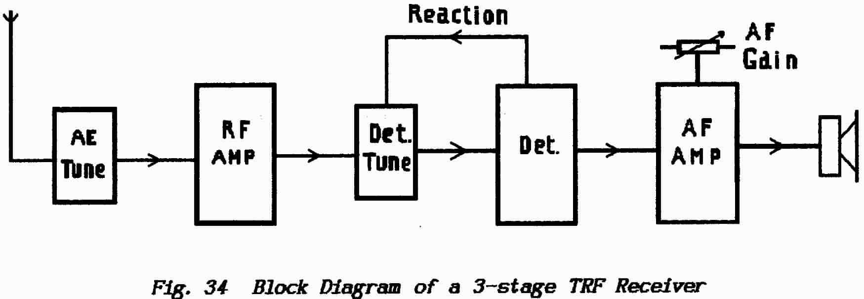
>>>>>>>>>>>>>>>>>>>> PAGE 73 <<<<<<<<<<<<<<<<<<<<
** TRF receivers have been built using more than one rf-amp and often an audio-amp is added partly to increase the overall sensitivity but mainly to provide the necessary signal level to drive the power amplifier. Placing several rf-amps in cascade leads to a circuit arrangement wherein amplifiers have tuned circuits at both their inputs and outputs ; such a circuit is described in Part 4: Electronic Oscillators as the tuned-anode-tuned-grid (T.A.T.G.) oscillator.
** The problem of oscillation in the multistage rf-amp is further complicated by the need to tune each of the resonant circuits simultaneously if the receiver is to operate over a band of frequencies. See also under 3.13.13: Decoupling .
** Most of the problems with TRF receivers stem from the need to tune them over a band of frequencies but it is a problem with all receivers that bandwidth, selectivity and sensitivity change with the tuning.
** Clearly the difficulties can be designed away for a receiver that is to operate at a fixed frequency. All modern receivers endeavour to get the best of both worlds by using a receiver in which the main body operates at one frequency only in combination with a front-end that can be tuned over any desired band but whose output is always at the frequency of the fixed receiver. (See Superhet receivers in Lesson 13.)
END OF LESSON 12
* * * * * * * * * * * *
QUESTIONS
1. Why are some communications receivers fitted with an aerial attenuator?
2. Why do most domestic receivers not employ an rf-amplifier?
3. What tasks does the Demodulator perform?
4. In what ways do domestic and communications receivers differ?
5. If a receiver is unable to resolve a weak signal when other receivers can cope where would you suspect the trouble to lie?
6. State briefly the problems encountered with a TRF receiver and outline the steps proposed for their solution,
7. A capacitance of 0.1 µF is connected in series with one of 0.033 pF. What is the effective capacitance of the combination?
8. The above series combination of 0.1 and 0.033 µF is connected across a choke of 1 H. What is the resonance frequency of the resulting circuit?
9. How would you express the bandwidth of a circuit which passes frequencies from 460.5 kHz to 469.5 kHz ?
>>>>>>>>>>>>>>>>>>>> PAGE 74 <<<<<<<<<<<<<<<<<<<<
The previous Lesson ended with the observation that many of the ailments of a simple receiver can be overcome with fixed-frequency working. The superhet receiver uses this principle together with a tuneable front-end.
The name is a contraction of supersonic heterodyne which means that a supersonic (above audible range) beat-note is obtained by heterodyning (beating) the incoming carrier with another signal. The carrier-frequency of each required incoming signal is translated to a common carrier-frequency . (See Lesson-3, Funds-2.)
The bulk of the receiver, that which sets the gain and bandwidth of the overall system, is constructed as a fixed-frequency unit. The front end contains a variable oscillator (the local oscillator) which is tuned so that its frequency always differs from that of the desired incoming carrier by a constant amount. The output from the front end thus always contains a component — a beat note — with a frequency that is constant whatever carrier the front end is set to receive.
In domestic receivers the front end seldom consists of more than the frequency-changer stage together with the aerial-tuning coil and the variable local oscillator. Its output is usually in the region of 465 kHz. Communications receivers invariably incorporate one or more rf-amplifier stages before the frequency-changer stage and a variety of output frequencies are used depending on the purpose of the receiver.
The fixed-frequency output from a frequency-changer is referred to as the intermediate frequency or the I.F. because it is intermediate between the rf carrier-frequency and the final audio frequencies.
The fixed-frequency part of a superhet receiver operates at the intermediate frequency and so is usually known as the i.f. unit, i.f. amplifier, i.f. stages or simply as the i.f. It is too often forgotten however that the i.f. is, in fact, the receiver proper. Fig. 35 shows the basic block diagram of a typical superhet receiver.
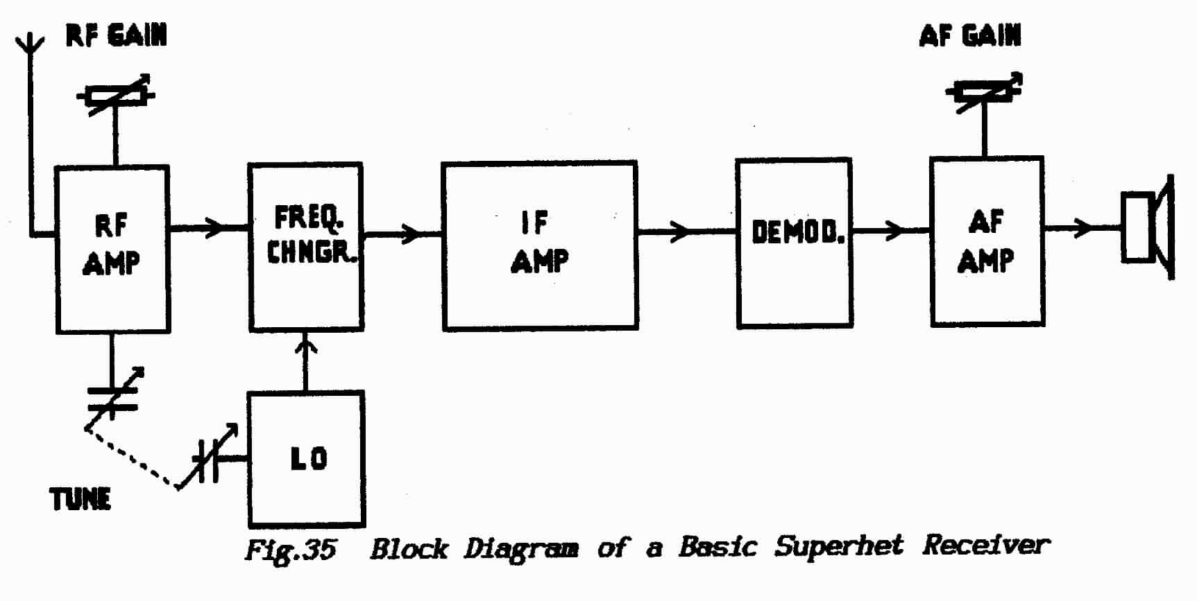
>>>>>>>>>>>>>>>>>>>> PAGE 75 <<<<<<<<<<<<<<<<<<<<
As shown in Lesson-3 of Part-2 frequency-translation requires that a carrier is mixed with another signal of suitable frequency in a non-linear circuit. Such a non-linear circuit can be a diode (either thermionic or semi-conductor) which is a two-terminal device that conducts in one direction but not in the other. Although at uhf and higher frequencies there is often no alternative to a small diode the technique is seldom found in domestic or communications receivers because other methods provide a larger i.f. output. The ratio of if-signal output to rf-signal input is known as the conversion gain.
It is usual to use a valve or transistor-device as the non-linear mixer and there are many such devices and as many more circuit arrangements. As indicated in Lesson-3, frequency-changers (or mixers) come in two basic forms namely additive mixers and multiplicative mixers. As a guide the rf and L.O. signals are added to the same input of an additive mixer but to different inputs of a multiplicative mixer.
A disadvantage of additive mixing is that, unless the added complication, and cost, of a buffer stage is used after the local-oscillator, the L.O. has a tendency to "pull" into step with the carrier signal; this tendency is resisted at the higher frequencies by raising the i.f. frequency which increases the separation.
There is a problem fundamental to all mixer stages in that the local-oscillator tuning must be kept at all times a fixed interval either above or below that of the required incoming carrier-frequency. At a first glance this may appear a simple matter but unfortunately it is not so.
Consider a tuneable receiver that is to work over a band from 1 to 2 MHz with an intermediate frequency of 100 kHz. The local oscillator might be either above or below the signal frequency and so we have:
Signal Range: 1 to 2 MHz or 1.5 MHz ± 0.5 MHz
Local Oscillator high 1.1 MHz to 2.1 MHz or 1.6 MHz ± 0.5 MHz
Local Oscillator low 0.9 MHz to 1.9 MHz or 1.4 MHz ± 0.5 MHz
which seems straightforward enough ?
However the tuning range of a variable capacitor is from its minimum to its maximum capacitance irrespective of the centre frequency which is chosen by selecting the inductance. The parameter of interest here is the amount that the frequency has to change as the capacitor is moved between minimum and maximum settings. In the Table above it is not the range of ± 0.5 MHz that matters but the comparison between that figure and the centre frequency. Thus:
at 1.5 MHz a range of ± 0.5 MHz represents a change of ± 33.33%
at 1.6 MHz a range of ± 0.5 MHz represents a change of ± 31.25%
at 1.4 MHz a range of ± 0.5 MHz represents a change of ± 35.7%
This shows that, with the local oscillator operating above the frequency range of the incoming signal, it must tune over a lesser range while, with the local oscillator operating below the range of the incoming signal, it must tune over a greater range.
>>>>>>>>>>>>>>>>>>>> P76 <<<<<<<<<<<<<<<<<<<<
Tuning several resonant circuits simultaneously with the one knob is achieved by use of "ganged" variable capacitors; i.e. several of these units mounted on a single rotating shaft. The immediate requirement for a superhet receiver therefore is a multi-gang capacitor in which one section has either a reduced or an enhanced range of capacitance.
Indeed this solution has been used by many manufacturers but it is a costly solution and one that is still subject to pitfalls; e.g. the actual range achieved by a variable capacitor is determined by the stray capacitances which shunt it and so, to use a specially-made component, it becomes necessary to control the strays.
Inevitably some kind of trimming is required to bring all the resonant circuits into tune with each other and the usual solution adopted is to use a ganged capacitor in which all the units are identical and to "trim" the range electrically.
One method of reducing the range is simply to place a fixed capacitor across the variable thus reducing its relative range. However this involves an increase in the total capacitance and so the value of the inductance must be changed. The end result of such a simple arrangement is lack of tracking the accepted term for keeping the rf-circuits and the L.O. circuit tuned in. step.
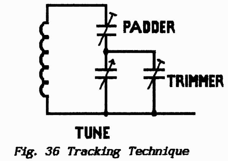 |
The usual technique is illustrated
in Fig.36. A small variable trimmer capacitor
is connected in parallel with the L.O. section of the ganged capacitor
and a second much-larger variable padder capacitor
is connected in series.
At high-frequency settings, where the main capacitor is set to its minimum value, the trimmer increases the minimum capacitance and so restricts the upper frequency-limit; the (relatively-large) series-connected padder makes very little difference to the combined capacitance. At the low-frequency settings, where the main capacitor is set to its maximum value, the series-connected padder reduces the |
maximum capacitance and so restricts the lower frequency-limit; the (relatively-small) parallel-connected trimmer makes very little difference to the combined capacitance.
** There are two important points which are likely to be
(i) because this technique restricts the tuning range at both ends it is necessary to set the L.O. to work above the incoming carrier frequency.
(ii) because the trimmer and padder perform their tasks under different conditions they make it possible to tailor the relation between capacitor-setting and the resulting frequency.
Although the trick can be made to work very well it nevertheless is not a perfect solution. The actual received frequency which is passed to the i.f. unit is determined by the L.O. setting; the failure to achieve perfect tracking is not important provided that, as a result, the rf-signal circuits are not required to operate outside their bandwidths. This is a matter of design compromise.
>>>>>>>>>>>>>>>>>>>> PAGE 77 <<<<<<<<<<<<<<<<<<<<
The tracking is usually adjusted at points roughly 20% from each end of the range after which it drifts back and forth as the tuning is varied across the band.
(a) Image or Second-channel Interference
As given in the previous Section the frequency of the local oscillator in a superhet receiver is always higher than the required signal frequency by an amount equal to the required i.f. frequency. However there is another frequency, higher than the L.0. signal by the same amount, that is able to beat with the L.0. to produce the designed i.f.; this frequency is separated from the required frequency by twice the intermediate frequency and is known as the image frequency.
Should a signal be present on such a frequency then, provided it is strong enough to overcome the discrimination of the r.f. stages, it too will send an if-signal to the I.F. section of the receiver and the two signals cannot be separated thereafter. The interference which this causes is known as second-channel interference or sometimes as image interference.
The only way to eliminate this nuisance is to prevent signals on the image channel reaching the frequency-changer. This is one of the reasons (a major reason) for placing one or more rf-stages in front of the mixer stage. But once again the solution is not so simple as it may seem.
An amateur receiver operating on 14 MHz with an I,F. of 100 kHz may have an interfering station putting in a powerful signal on its image channel at 14.2 MHz; i.e. 200-kHz higher. This is a very good separation as far as the likely bandwidth of either signal is concerned. However, in terms of asking the rf-amplifiers to eliminate 2nd-channel interference, the separation is 200-kHz in 14-MHz which is about 1.4% -a very tall order especially for a variable-tuned circuit.
The answer here is to raise the intermediate frequency. An i.f. of 1-MHz would put the image channel at 16-MHz and increase the separation for the rf-amps to 2 MHz in 14 MHz or 14%.
(b) Adjacent-channel Interference
As the name implies this is interference caused by stations on frequencies so close to the required frequency that the tuned circuits of the receiver cannot separate them. Narrow-bandwidth circuits are not very difficult to design but to make them narrow and also tuneable is all but impossible within reasonable cost. It is here that the superhet principle really shines.
The I.F. stages of the receiver operate at a fixed frequency and so the design parameters for this part of the equipment can be chosen for optimum performance. To get the steep edges (or skirts) to the passband which is required if adjacent-channel signals are to be eliminated requires use of the bandpass circuits which were introduced in Fundamentals-1 Lesson-10.
Once again the separation of two signals depends on there being a significant difference in their frequencies as a percentage of their centre-frequency. It follows therefore that, to remove signals that are separated from the wanted carrier by 3-kHz (or even less), requires the i.f. to be kept low and a value of 100 kHz is not unusual.
>>>>>>>>>>>>>>>>>>>> PAGE 78 <<<<<<<<<<<<<<<<<<<<
Section 2.7.3 shows that the successful construction of a superhet receiver has two conflicting requirements; a high i.f. to eliminate image-channel problems and a low i.f. to eliminate adjacent-channel problems. Fortunately the superhet principle itself provides an ideal answer.
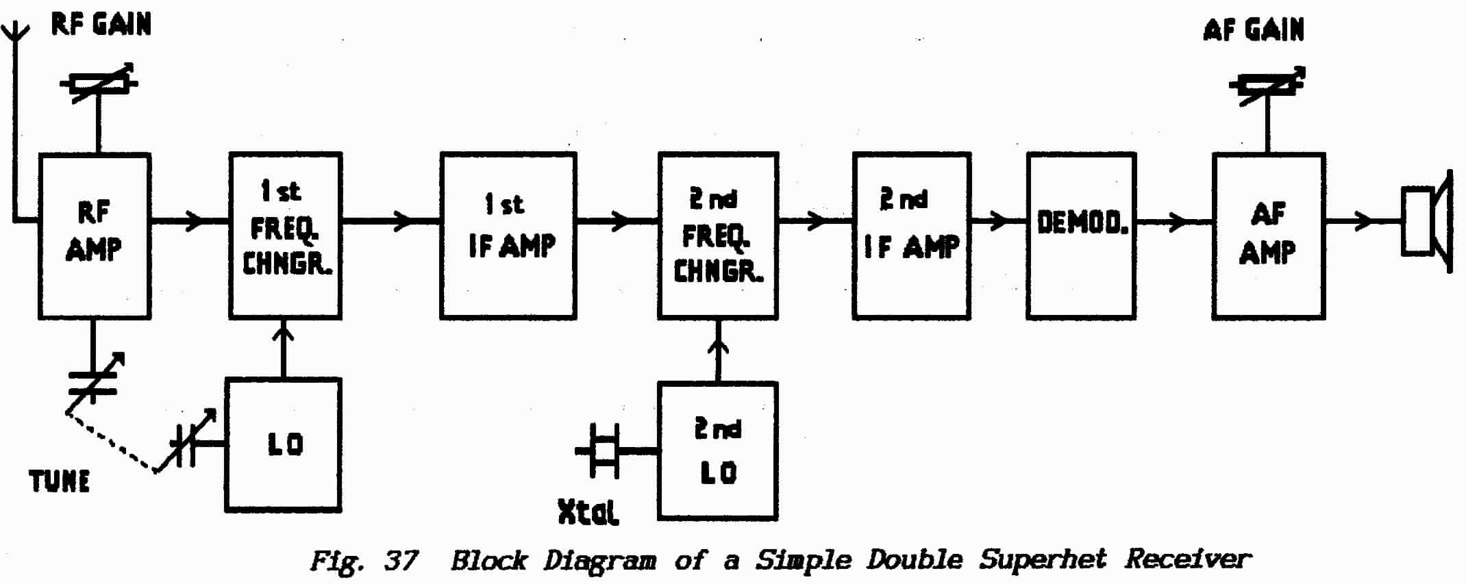
As shown in Fig.37 the double-superhet performs the frequency-changing act twice and uses two intermediate-frequencies in two cascaded if-amplifiers (they follow each other). The first i.f. is set as high as practicable so as to remove the image-channel from consideration. The second i.f., now protected from image interference, is made as low as practicable so that its bandwidth can be made very small to eliminate adjacent-channels.
For technical reasons beyond the scope of these Lessons the principle is sometimes extended further to a triple-superhet. Note however that the Racal receivers, which use the Wadley Loop and which are often described as triple- superhets, are in fact double-superhets; these receivers are much misunderstood. (See later in this Section.)
The frequency-changer stage is often referred to as the first detector which reflects its non-linear task in extracting the intermediate frequency. In a double-superhet the second frequency-changer stage becomes the second-detector. The final detector stage, that which extracts the modulating signal, is known as either the second-detector or third-detector as appropriate.
In the double superhet receiver the second local-oscillator operates in conjunction with the fixed frequency of the first-i.f. and consequently it does not need to be tuneable. It is usually a crystal-controlled oscillator.
Problems with superhet receivers are unique to the technique and consist mainly of a series of whistles hums and noises which, very often, are extremely difficult to trace and eliminate.
>>>>>>>>>>>>>>>>>>>> PAGE 79 <<<<<<<<<<<<<<<<<<<<
A good starting point is to note that any signal with a frequency within the i.f. passband, which reaches the input to the i.f. unit, will appear at the receiver output. Such a spoof i.f. signal can be derived from:
(a) image-channel and adjacent-channel signals as described above
(b) two signals beating together whose frequency-separation is equal to the i.f. frequency or where they produce harmonics with that separation; this problem occurs mainly with additive mixers.
(c) any signal whose carrier-frequency is separated from a local-oscillator harmonic by an amount equal to the i.f. frequency
(d) any harmonic of a carrier-signal which is separated from the local-oscillator frequency by an amount equal to the i.f. frequency
(e) by combining c and d above wherein a beat at if-frequency is set up between a harmonic of a carrier-signal and a harmonic of the local-oscillator
(f) a harmonic of the i.f-signal which manages to arrive back in the rf-circuits and beats with a harmonic of the local-oscillator.
(g) an rf-carrier at or close to the i.f. frequency which is permitted to reach the input of the frequency-changer.
That is enough to demonstrate the facility with which a superhet receiver can be difficult. The problem of whistles is greatly exacerbated by the fact that the strength of the resulting beat note is dependent on the power of EITHER of the carriers involved. Thus only one of the inter-acting signals needs to be strong.
The sources of the harmonics mentioned above are not difficult to identify although, in practice, they can be very difficult to trace; they can be generated in any non-linear circuit within the receiver. This can result from a straightforward overload by a too powerful signal or because a powerful signal has developed a large a.g.c. bias which is over-enthusiastic in reducing the receiver gain. Hence the need for an aerial attenuator. Many problems are caused by insufficient isolation between the aerial circuits and the i.f. amplifier and by unwanted signals invading the local oscillator or escaping from the local oscillator.
In the discussion above the point was made that the local oscillator in the frequency-changer stage operates of necessity at a frequency above that of the incoming signal. This point is stressed in the R.A.E.
It is worth noting however that there are two circumstances in which the rule may be waived:
(i) In a double superhet the second L.O. can be placed either above or below the first-i.f. frequency because the L.O, operates at a fixed frequency and so tracking problems do not arise.
(ii) The rule holds for all-band (General Coverage) receivers but not for receivers which cover only limited bands. Amateur receivers for example, especially those which are incorporated into Transceivers, cover only the frequency ranges permitted by the amateur- licence;
>>>>>>>>>>>>>>>>>>>> PAGE 80 <<<<<<<<<<<<<<<<<<<<
the greatest relative bandwidth here is that from 3.5 MHz to 3.8 MHz (about 8 %). Over such a limited range a loss of tracking would not be important and so the L.O. could be placed on either side of the incoming carrier as dictated by other considerations. This can be beneficial where the first i.f. is set very high; for example, should it be decided to place the 1st-if at 10.7 MHz then, to cover the 3.5-MHz Band, the L.O. must cover from 14.2 MHz to 14.5 MHz or from 7.2 MHz to 6.9 MHz. It is much easier to deal with an oscillator operating on 7 MHz than with one operating on 14 MHz.
Modern "black-box" transceivers are fitted with an IF-Shift control. This can be very useful in cw working to eliminate a powerful adjacent-channel signal by pushing it "over-the-edge" of the if bandpass characteristic. The BFO is set to whichever side gives the unwanted signal the higher pitch and then the IF is shifted until the unwanted signal is attenuated. In fact, to make a bandpass if amplifier with a tuneable characteristic is very expensive and most unlikely to be satisfactory as a long-term strategy. With a double superhet however all that is necessary is to drift the frequency of the (nominally-fixed frequency) 2nd L.O.; in other words it is not the if-amp which is shifted relative to the if carrier but the carrier which is shifted relative to the if-amplifier.
This technique is most successful in double superhet receivers because of the relatively-narrow bandwidth of the 2nd-if amplifier.
END OF LESSON 13
* * * * * * * * * * * *
QUESTIONS
1. What is the basic difficulty which is overcome by the complication of using the superheterodyne principle?
2. What is the basic difficulty which justifies the use of a double-superheterodyne design?
3. Why do you not find tuneable superhet receivers in which the local-oscillator output is set below the carrier frequencies?
4. What design features would you expect to find in an i.f, unit?
5. In a double-superhet receiver where would you expect to find the beat-frequency oscillator for c.w. reception?
6. For a good technical reason a receiver is to have an i.f. of 10.7 MHz but it is required to tune over the continuous range 10 to 12 MHz. Clearly, at the lower end of this working range, the rf-input will gain direct access to the frequency-changer input. In broad terms only, can you suggest a technique for preventing trouble?
7. Explain the terms frequency-translation and frequency-multiplication.
>>>>>>>>>>>>>>>>>>>> PAGE 81 <<<<<<<<<<<<<<<<<<<<
** An rf-amplifier provides gain to raise signal-level from the very small value delivered by an aerial to one more suitable to drive the following stage be it a frequency-changer or a demodulator. However, gain of itself is not the main reason for employing one or more rf stages; low signal-level can often be overcome by other arrangements such as the leaky-grid detector described above.
** The real benefit of rf-amplification is that each stage introduces an extra tuned circuit and so increases the selectivity. As described in the previous Lesson good selectivity before the frequency-changer is necessary to eliminate 2nd-channel interference.
** Of course, any form of enhanced selectivity will also provide a measure of protection from adjacent-channel signals but such is not part of any design intention because the rf-circuits must be tuneable and so they will exhibit variable bandwidth.
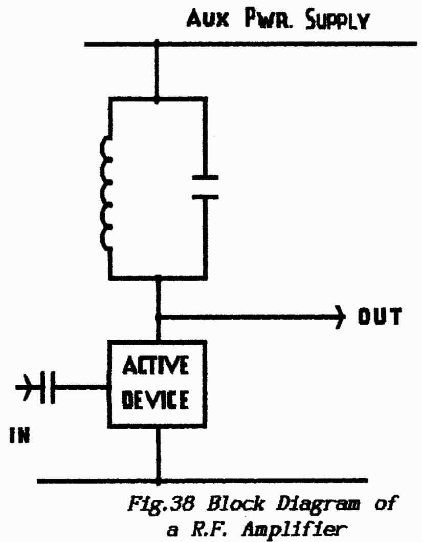 |
** A typical rf-amplifier is shown in block form in Fig. 38. The input, via the coupling capacitor, may come from an aerial-coupling coil or from the output circuit of a previous rf-amplifier. The output load, through which the amplifier drives its output current, is a tuned-circuit. This presents its highest impedance at the frequency to which it is resonated and so develops the maximum output voltage at that frequency. In this way an rf-amplifier discriminates against unwanted carriers. ** A well-designed and constructed amplifier allows the passage of rf signals from its input to its output (amplifying them on the way) but does not transmit such signals in the opposite direction. An rf- amplifier thus prevents output from the local-oscillator reaching the aerial. An important function of the first rf-amplifier (the very first stage of a receiver) is that it controls the noise performance of the receiver. incoming from the aerial the ratio of signal-amplitude to background noise can be adjusted only in the design of the aerial system; it cannot be altered in the following receiver. However, it is a fundamental concept that any receiver must inevitably add its own quota of noise and so it unavoidably degrades the incoming signal-to-noise ratio. The point most vulnerable to noise in a receiver is the aerial input where the signal is at its lowest value; from there on the receiver amplifies equally both signal and noise. Thus it is important to design the first stage so that it adds as little noise as possible |
It is normal to make the input impedance of a receiver 75-ohms so that it matches the low-power coaxial cables usually used to connect a receiving aerial.
>>>>>>>>>>>>>>>>>>>> PAGE 82 <<<<<<<<<<<<<<<<<<<<
** Where the receiver is part of a combined transmitter/receiver equipment (a transceiver) then the receiver input-impedance is the same as the transmitter output-impedance which is normally 50-ohms. In Fundamentals- 1, Lesson 11 it was pointed out that there is advantage in making the input-impedance of a receiver higher than that of the connecting feeder. Circuit details of rf-amplifiers and aerial connections are given in Part-3 of this Course.
** Essentially if-amplifiers and rf-amplifiers do not differ except that the if-amplifier operates at a fixed frequency. The i.f. section of a receiver has two principal functions:
(a) it provides the major part of the receiver amplification
(b) it uses band-pass circuits to eliminate adjacent-channel interference while preserving the balance of the side-frequencies.
The passband requirements depend on the use for which the receiver is intended. For domestic "music" a.m. reception the passband ought to be adequate to accommodate the side-frequencies which result from a full audio bandwidth; i.e. 50 Hz up to 15 kHz. However the great demand for channels means limiting the channel separation to around 9 kHz and so the bandwidth of the if-amps is usually around ± 7.5 kHz, (Remember that bandwidth is specified at the 6-dB points where the signal strength has been reduced by one-half.).
** Communications receivers however are not concerned with faithful sound reproduction but require that the signal should be read as easily as possible. The noise which a receiver both picks-up and generates is directly proportional to the bandwidth and so the design of communications receivers aims to restrict the bandwidth as much as possible.
** For phone operation audio bandwidth is restricted to "telephone" quality about 300 Hz to 3.5 kHz. For a full double-sideband a.m. signal this would require an i.f. band of frequencies extending to 3.5 kHz either side of the carrier frequency. For single-sideband (ssb) operation, the bandwidth required in the i.f. is just 3.5 kHz starting from the carrier frequency and extending upward (for upper-sideband working) or downward (for lower-sideband working).
** For c.w. working however, where only the carrier frequency is involved, the bandwidth can be drastically reduced and this eliminates much of the background noise together with most of the adjacent-channel interference. There is a lower limit to i.f. bandwidth which is set by the stability of the local oscillator(s). Drift in these causes drift in the frequency of the i.f. signal and clearly this signal must remain within the passband of the i.f. amplifier.
It is not unusual for communications receivers to offer a (selectable) bandwidth as low as 300 Hz but use of this setting depends not only on the stability of the oscillators concerned but also on the skill of the Operator in setting-up the receiver. The front-end of Racal receivers (mentioned earlier) make use of a circuit configuration known as the Wadley Loop which eliminates the effects of oscillator drift; consequently these receivers offer an additional bandwidth of 100 Hz to those with the operational skills to adjust the receiver.
** Variable bandwidth or, to be more accurate, switch-selectable bandwidth is usually provided in the i.f. unit. There are two basic methods:
>>>>>>>>>>>>>>>>>>>> PAGE 83 <<<<<<<<<<<<<<<<<<<<
(a) set the i.f. bandwidth to at least the greatest value desired and switch in filter networks to reduce it as required
(b) vary the bandwidth of the bandpass circuits by changing the damping (see Lesson 10 under 1.14.3); this cannot be done when using stagger-tuned circuits.
** The design and construction of variable bandwidth circuits is not dealt with in this Course. The use of crystal filters may be touched on in the R.A.E. however. All that is required is that bandpass-circuits can be constructed with very steep skirts and also with very narrow bandwidths by using crystal (quartz) resonators in place of, or in conjunction with, the normal i.f. tuned circuits. Some filters use mechanical resonators in place of the quartz crystals. Normally such filters are bought ready made. Some early receivers used a single crystal together with a phasing control which effectively re-balanced the circuit to compensate for the introduction of the crystal.
Note that when using frequency modulation the bandwidth required is determined by the deviation and the modulation index and not necessarily by the bandwidth of the modulating signal; see Lesson-2 of this Circuit details of i.f. amplifiers are given in Part 3.
** The function of the demodulator stage is to accept the modulated signal from the last i.f. amplifier stage and to extract from it the modulated information. In a modern multi-purpose receiver this stage may have to cope with double-sideband am signals (domestic broadcast programmes), ssb, fm and cw.
(a) C.W. Signals
** C.W. transmissions use only a keyed carrier. To make this audible at the receiver output the i.f. signal is heterodyned with a local oscillator (the Beat-frequency-oscillator). It is usual to set this B.F.O. nominally to the centre i.f. frequency and to provide a control that shifts it either up or down by about 5 kHz.
** The signal presented to the detector varies in amplitude at the difference (beat) frequency (see Lesson 3 of this Part) which, after detection, is heard as an audible beat-note whose pitch can be adjusted by the B.F.O. control.
** That the B.F.O. can be shifted either up or down in frequency is an important facility. Where an interfering signal is on the same frequency as the desired signal it is not possible to separate them and only the morse-operator's skill can save the day. More usually such an interfering signal is not exactly on the same frequency and its separation can be increased by shifting the B.F.0. to the "other side" of the wanted carrier. Separation is also aided by adjusting the B.F.0. so that the desired signal produces the more insistent sound or by arranging that the beat with the unwanted signal is outside the audio bandwidth. Selectable or adjustable audio filters are a great help in such a situation.
(b) A.M. Signals
** A normal carrier is a continuous sine-waveform which makes equal excursions above and below zero ; its average value over a period of several cycles is zero. When such a wave is modulated by varying its amplitude the average value remains at zero as the crest values, both positive-going and negative-going, are varied.
>>>>>>>>>>>>>>>>>>>> PAGE 84 <<<<<<<<<<<<<<<<<<<<
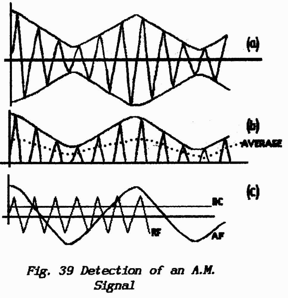 |
** Such a modulated wave is shown in Fig.39(a) with
the base (zero) line as the average value. In diagram (b) the lower half
of the modulated waveform has been removed; as shown the average
value of the discontinuous waveform which is left follows the modulation
waveform as indicated by the carrier envelope.
This form of demodulation requires a rectifier or detector in the form of a diode which permits current-flow in one direction but not in the other. The direction of flow is a matter of which way round the device is connected into the circuit and that is decided by the requirement either for a positive-going or a negative-going output. ** The output from such a detector is a varying direct-current which, as shown in diagram (c), can be analysed into an ac audio signal, an ac carrier signal and a dc bias. These are separated, usually by use of a capacitor, and the audio ac-signal is passed to the audio amplifier; the residual carrier is filtered out. |
** The value of the dc depends on the amplitude of the modulated carrier before the detection process; this dc-signal is used to operate the automatic gain-control (a.g.c.) system which is described later.
(c) SSB Signals
** As described in Fundamentals-1 a suppressed-carrier signal is without a carrier component and the waveform of the combined side-frequencies constantly reverses phase. To recover an undistorted modulation signal it is necessary to re-insert the carrier and this has to be done with considerable precision both in frequency and in relative amplitude. In theory the reconstituted signal is then processed as a double-sideband signal.
** A single-sideband signal must undergo essentially the same process but of course one set of side-frequencies is absent. The process is usually carried-out in one stage using one of the forms of ring-modulator or balanced modulator operated "in reverse". In most transceivers the same circuit is pressed into operation both as a modulator while transmitting and as a demodulator when receiving. Details of these circuits are described in Part 3 of this Course.
It is possible to demodulate an ssb signal using a communications receiver which is not suitably equipped by setting-up the c.w. local-oscillator (the beat-frequency oscillator or B.F.O.) as a carrier-insertion oscillator. This is not an easy option however; it requires good frequency stability from the oscillator and a slow-motion drive to allow accurate adjustment of its frequency. Additionally it is necessary to juggle the rf-gain and aerial-attenuator controls to obtain the correct relative amplitudes of ssb signal and local oscillator. Of necessity the local-oscillator must be adjusted to the correct side of the ssb signal, dependent on it being an upper-sideband or lower-sideband signal, and the receiver must be set for a.m. reception.
>>>>>>>>>>>>>>>>>>>> PAGE 85 <<<<<<<<<<<<<<<<<<<<
(d) F.M. Signals
** The modulation component is extracted from a frequency-modulated signal by means of a circuit called a discriminator. According to its method of operation it may be referred to as a slope detector, ratio detector, Foster-Sealey discriminator and others.
** Essentially these circuits produce two i.f. outputs which are combined so that the overall output signal is proportional to the frequency of an applied carrier. (We say that the circuit is made frequency conscious). Thus, as the carrier frequency is varied by the modulation, the signal is converted to amplitude + frequency modulation. The f.m. is then ignored and the modulation detected as with an a.m. signal; these circuits are described in detail in Part 3 of this Course.
** It is usual to over-drive the active device which feeds the discriminator so that this stage acts also as the Limiter. Most of the noise, both incoming and self-generated within the receiver, is in the form of amplitude-modulation and the limiting action removes all amplitude variations thus producing the extremely-quiet background which is a feature of f.m. transmissions.
It is possible to receive f.m. transmissions with a communications receiver that is not fitted with a discriminator. With the B.F.O. switched off and the a.m. mode selected the receiver is detuned so as to bring the required signal on to the skirts of the i.f. bandpass circuits; this makes the i.f. amplifier frequency-conscious so that the i.f. signal, which is presented to the detector, changes amplitude with the variations in frequency.
Once again however the trick is not easy to achieve. The bandpass circuits have steep skirts which may not facilitate either the full swing of the modulated carrier or drift in any of the superheterodyne oscillators. This can be offset by selecting a wide bandwidth setting - with all the disadvantages of wide bandwidth. The conversion of f.m. to a.m. is not likely to be very linear and so considerable distortion is to be expected. Above all the a.m. receiver is not fitted with a Limiter stage and so a considerable amount of noise is to be expected also. Possibly the greatest limitation is the available accuracy in tuning so as to place the nominal carrier-frequency in the centre of the i.f. skirt.
When attempting to receive f.m. signals in this manner the automatic gain-control (a.g.c.) should be switched off. Much depends on the filtering in the a.g.c. line but, with the receiver de-tuned, the signal at the detector stage is likely to be fairly weak, the r.f. and i.f. stages will be operating around their full gain and any audio which gets into the a.g.c.
The A.F. Amplifier performs three functions:
(i) Amplifies the low-level signal from the demodulator
(ii) Provides the power necessary where it is desired to operate with a loudspeaker
(iii) Provides an Audio Gain control which is used to set the post-detector gain as determined by the noise output from the detector with weak signals
>>>>>>>>>>>>>>>>>>>> PAGE 86 <<<<<<<<<<<<<<<<<<<<
It is not generally realised that full-band audio amplifiers are difficult to design arid can be a source of considerable trouble; as shown in Lesson-1O of Fundamentals-1 an audio amplifier has by far the greatest relative bandwidth. However, as far as communications receivers are concerned, the audio amplifier is restricted in bandwidth and in gain and it is not required to produce "high-fidelity" sound.
** It is not uncommon nowadays to use audio filters although these are often built-in to a separate loudspeaker unit. Use of a narrow bandpass filter can greatly reduce the post-detector noise and those persistent adjacent-channel transmissions which often seem determined to have their say. Alternatively a so-called "notch" filter, which can be tuned across the audio band, can be used to attenuate such an unwanted signal. There is no reason of course why both should not be used simultaneously.
Such audio filters were possible at one time only by use of heavy and bulky iron-cored inductors. The advent of semiconductor operational amplifiers has made it possible to construct compact and easily tunable active filters; these are described in Part 3 of this Course.
END OF LESSON 14
* * * * * * * * * * *
QUESTIONS
1. In what manner do the if-amplifiers differ in domestic and communications receivers?
2. In cw-working, where side frequencies are generated only at the start and finish of each Morse character, there is benefit in restricting the bandwidth of a receiver. What is the benefit obtained, where can the bandwidth restriction take place and what limits the usable bandwidth?
3. (a) How is so-called variable bandwidth achieved?
(b) How are very narrow bandwidths achieved?
4. How does the recovery of the modulation from an f.m. carrier differ from other forms normally found in a communications receiver?
5. What is most important in demodulating a s.s.b signal?
6. What is a PLL ?
7. While working cw interference is coming in from two separate stations which are sitting nearly on top of your contact's signal. Detuning the receiver improves matters with one of them but always seems to make matters worse with the other. Is there some other technique which you could try?
8. Why should you not connect a dipole to a transmitter via a coaxial cable ? Many amateurs do this and seem to get good results; why is this?
>>>>>>>>>>>>>>>>>>>> Page 87 <<<<<<<<<<<<<<<<<<<<
Because i.f. amplifiers operate at a fixed frequency it is possible to use bandpass circuits in their construction. However, to achieve narrow bandwidths with very steep skirts, it is necessary to use several such i.f. stages in cascade. The number of stages required (ignoring considerations of gain) can be reduced by making use of the high-Q properties of crystal resonators. Many amateurs use old valve-operated receivers in which the single-crystal crystal-gate circuit is often found.
(a) Single Crystal or Crystal-gate Circuit
Pig.40 shows an i.f. transformer with a centre-tapped secondary which supplies, with respect to earth, two outputs of opposite phase. In some circuits it is not the inductor that is centre-tapped but (effectively) the capacitor by using two variable capacitors as shown in diagram (b).
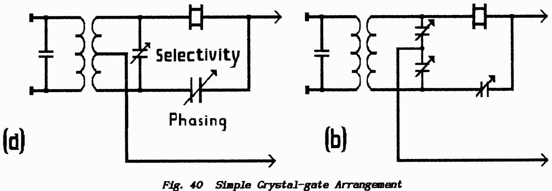
Both outputs are connected to the following stage one via a crystal and the other via a small variable capacitor. At a frequency well-removed from the resonance frequency of the crystal (where the crystal is ineffective) a signal is injected and the variable capacitor (the phasing capacitor) is adjusted so that its capacitance equals that of the crystal holder plus strays; a sharp null in the output shows that the two now-equal and opposite signals cancel.
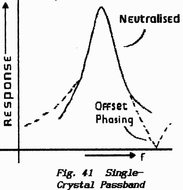 |
At the series-resonance
frequency of the crystal this circuit balance is disturbed by the crystal's
low impedance, cancellation fails and a signal appears at the output. Under
these conditions the circuit produces a high-Q passband similar to that
of the crystal alone.
A useful variation is obtained by altering the setting of the phasing-capacitor. Not only does this upset the balance but it introduces a small phase-error with the result that a point of complete cancellation (a notch) appears on one side of the passband as shown in Fig.41. This notch is moved to the other side of the passband when the phasing capacitor is shifted in the opposite direction. |
>>>>>>>>>>>>>>>>>>>> PAGE 88 <<<<<<<<<<<<<<<<<<<<
This notch can be very useful in removing an interfering adjacent-channel signal but there is a penalty in that the selectivity is degraded on the non-notch side.
A similar effect can be obtained by leaving the phasing capacitor undisturbed and varying the position of the tap. This is not practicable with a tapped inductor but can be arranged in Fig. 40(b) by varying the two capacitors differentially, i.e. by increasing one and decreasing the other so that the overall value remains constant.
The selectivity of the crystal gate can be varied by adjusting the tuning of the if transformer which drives it; the effect arises from the change in the dynamic
(b) Double Crystal Filter
The double-crystal circuit uses essentially the same arrangement but there is a crystal in each output from the i.f. transformer. The two crystals have different resonance frequencies which are separated by the required bandwidth. Each crystal behaves exactly as in the single-crystal circuit but, in the frequency range between their resonances, the two outputs add and so produce a bandpass effect.
The two crystals produce much steeper cut-off slopes with the result that out-of-band signals suffer some 20-dB more attenuation (a factor of 10) than with the single-crystal circuit.
In the two-crystal arrangement of Fig.42 variation of the phasing capacitor produces a notch on each side of the passband simultaneously. To vary the bandwidth it is necessary to switch between filters.
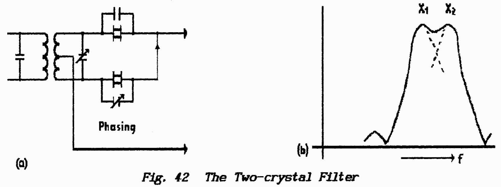
In superheterodyne reception an incoming carrier-signal is changed to a different frequency by beating it with the output from a local oscillator and detecting the result. In beat reception (or heterodyne reception) an unmodulated carrier is made audible by beating it against a local oscillator
>>>>>>>>>>>>>>>>>>>> PAGE 89 <<<<<<<<<<<<<<<<<<<<
whose frequency is close to that of the carrier frequency and again detecting the result. Autodyne reception is a form of beat reception in which the three functions of local-oscillator, mixer and detector are combined in a single stage. In some ingenious one-valve forms the resulting audio signal was reflexed (i.e. re-circulated) through the stage so that it acted also as an audio amplifier.
The homodyne (or synchrodyne) receiver takes the autodyne technique a step further in that the local-oscillation takes place at the frequency of the incoming carrier. The output from the circuit is the modulation waveform. The circuit can be viewed as a superheterodyne in which the i.f. carrier-frequency is zero. Once again reflex techniques were used to amplify the audio in a one-valve design.
To use this circuit in double-sideband reception however it is necessary to ensure correct phase-relation between carrier and the self-oscillation of the receiver. Needless to say, in both the above techniques, care is needed
** The dc receiver is most unfortunately named in that the initials stand for Direct Conversion. It is a natural development of the synchrodyne technique but, strictly speaking, it is not an autodyne circuit because it does not combine all the necessary functions in one circuit.
** The dc-receiver uses one of the ring-modulator or balanced-mixer type of circuits in a mode that can be regarded as a product detector (see later Lessons). In essence it reverses the modulation process; instead of applying a carrier and modulation waveforms and obtaining a modulated-carrier the dc-receiver applies a modulated carrier and an unmodulated carrier and derives the modulation waveform.
** Usually the detector is preceded by a simple rf stage, often untuned (i.e. broad-band) and followed by an audio filter and audio amplifier; these last two would most probably be combined in an active filter. The result is a very simple but often effective receiver. When incorporated into a transceiver the Transmit mode uses the demodulator in reverse as a modulator.
The lack of pre-detector selectivity and the susceptibility of the diode ring to overload renders the receiver useless in the presence of strong interfering signals in that it takes on the role of a broadband amplifier
This receiver technique is developed from the leaky-grid circuit with reaction that was described in Lesson 12. As discussed the sensitivity of the detector increases as the reaction is increased until self-oscillation sets in; maximum usable sensitivity occurs at that point.
>>>>>>>>>>>>>>>>>>>> PAGE 90 <<<<<<<<<<<<<<<<<<<<
The super-regen. circuit operates with the stage set for self-oscillation but the oscillation is quenched periodically by an imposed waveform that momentarily destroys the circuit loop-gain. The frequency of this quench waveform must be above the audio range (i.e. not less than 10 kHz) else it appears in the audio output as a high-pitched whistle. Equally the quenching frequency must not be too high else insufficient time elapses between quench-cycles for the stage to cease oscillation completely. Usually the range lies between 10 KHz and 100 kHz.
It is possible to arrange the circuit so that it squeggs (see later in Part 4: Electronic Oscillators). In this mode oscillation repeatedly stops and re-starts and so the circuit becomes self-quenching. A super-regenerative receiver offers poor selectivity and, without an incoming carrier, a high background noise; it also provides very-high sensitivity and excellent a.g.c. action. In general its performance all round improves as the carrier frequency is increased and it is at its most useful above 30 MHz.
Before the advent of semiconductors it was a popular device for radio-controlled models although its temperamental behaviour was responsible for spectacular failures. When a signal is detected the quench frequency changes and there is a significant increase of current drawn from the supply; this can be utilised to operate a relay or solenoid.
During WWII the circuit was developed to a high standard of reliability; if my memory is not at fault it was the basis of the airborne IFF Transponder (Identification Friend or Foe) which became necessary with the introduction of night-fighter aircraft. The self-quenching circuit can be adjusted so that it remains dormant until an interrogating signal appears on the frequency to which it is tuned; this triggers the quench circuit and the resulting bursts of oscillation radiate from the aerial as a response.
** The main purpose of any form of gain control is to adjust the output level for the comfort of the 0perator; normally this is the function of the AF Gain control. There is a secondary use in that strong signals fed into a high-gain receiver are likely to cause overloading in the high-level stages unless the gain is reduced in the early part of the receiver; this is the prime function of any RF Gain control. Note too that reducing gain in the early stages reduces the background noise level. It is unusual to provide a manual control of gain for an i.f. amplifier.
** The automatic control of receiver gain is normally applied only to rf and if amplifiers. Its two-fold purpose is to enable a receiver to be tuned between strong and weak signals without the need for constant gain adjustment and to reduce the unpleasant effects of signal fading.
** In Lesson-4 it was shown that one of the output components from an amplitude detector is a dc which is proportional to the carrier amplitude; for strong signals this dc component is greater than it is for weak signals and, when fading occurs, this component varies in step with the changes in signal strength. This dc-component is used as the output sample in a negative feedback-loop (see Lesson-5 in Fundamentals-1) whose function is to maintain a constant level of signal at the detector.
** The dc-output from the detector (the a.g.c. line) is connected to (some of) the rf and if stages, and often to the frequency-changers as well, as a bias which reduces the gain of these stages thus causing the pre-detector gain to fall as the signal strength increases.
>>>>>>>>>>>>>>>>>>>> PAGE 91 <<<<<<<<<<<<<<<<<<<<
It is necessary to grade the amount of feedback applied to each stage and also to leave some stages without a.g.c.; in the presence of a very strong signal the large a.g.c. bias which is developed could disturb the dc-working conditions of the active devices (see Part 3) and so cause serious distortion in those later stages where the signal has been amplified to large amplitude.
** A simple a.g.c. system, as shown in Fig.43 has a distinct disadvantage in that a feedback control-signal is always present and so even weak stations cause some reduction in gain. It would be better if the a.g.c. loop were to wait until the incoming signal reached a level that was approaching the maximum permitted at the detector and then began to restrict the gain so as to avoid overload effects. Such a control loop is referred to as Delayed A.G.C. In simple terms the dc component from the detector is inhibited by a bias voltage which keeps the a.g.c. line at ground potential until the dc-component exceeds the bias level. One method of adjusting the rf-gain is to vary this delay bias.
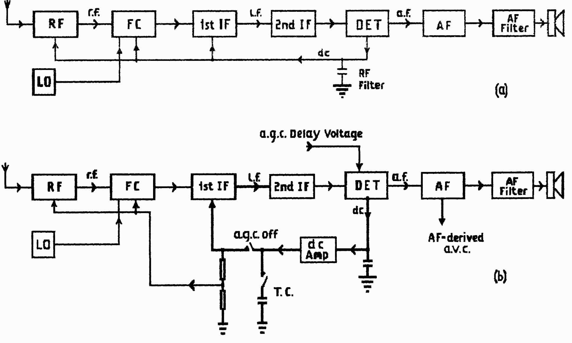
Fig.43 Block Diagrams of A.G.C. Systems
** The final if stage which drives the detector can be relieved of the necessity to supply a large output for a.g.c. purposes by interposing a dc-amplifier between the detector and the a.g.c. line. The extra gain introduced into the feedback loop makes the resulting Delayed Amplified A.G.C. very effective.
** In general, fm receivers are not fitted with an a.g.c. system because they use a Limiter and the full gain of the rf/if stages is utilised to ensure that this device is well and truly limiting. Nevertheless, where high gain is provided to enable the reception of very weak signals, it could be that a very-strong signal would swamp the limiter stage. Such receivers may tap the bias-potential developed in the limiter and feed this back to some of the earlier stages as an elementary a.g.c.
>>>>>>>>>>>>>>>>>>>> PAGE 92 <<<<<<<<<<<<<<<<<<<<
Any manual rf (or if) gain controls which fall within the a.g.c. feedback loop will be rendered inoperative by the a.g.c. action; thus, where manual gain-control is provided as an option, it is essential to provide an a.g.c. On/Off switch. This switch is also used in cw-working where the receiver uses a diode-type detector because this type of detector requires a high-level of b.f.o. output and this causes a large a.g.c. voltage which reduces the receiver sensitivity.
** In some receivers an a.g.c., signal may be derived from the audio output signal as a means of ensuring that the audio remains constant; this a.g.c. must be derived before the AF-gain control however if this control is to remain functional. Note that this technique maintains a constant-level of audio and so cannot be used for broadcast working where there is a requirement for receiving music.
[A large orchestra can produce a very-large dynamic range from very loud passages to very quiet. One of the main reasons that broadcast or recorded programmes never sound exactly like a "live" performance is that the dynamic range has to be limited because of problems with recording media and with transmitters. Despite constant manipulation of the sound level to maximise the effects of the musical dynamics a sudden crash of sound can overload a powerful transmitter and cause its protection circuits to shut-down the equipment. The necessary safeguards are provided by "Limiters" which utilise a form of a.g.c.]
** It is usual to find an A.G.C. Tine Constant (see Lesson 3, Funds.-1)) switch which, usually, is incorporated into a 3-position switch with the a.g.c. on/off. This varies the capacitance connected across the a.g.c. line so varying the time taken for the a.g.c. voltage either to rise to its final value or to die away again. In general the a.g.c. should respond quickly but not die away until it is certain that the signal has gone; usual attack and decay times are about 2 mS and 200-300 mS (milliseconds).
** When working cw there is the possibility of the a.g.c. circuit "remembering" the signals that have passed and adding them together so as to exaggerate the signal strength; with continuing morse the receiver gain would slowly decrease. In mathematical language we say that the a.g.c. circuit would integrate the morse symbols. This is avoided by decreasing the a.g.c. time-constant; hence the "fast" a.g.c. setting is used for morse and the "slow" setting for other voice working.
** The potential on the a.g.c. line is a direct indication of the incoming signal strength and the simplest form of tuning indicator therefore is a voltmeter which indicates this potential; tuning is adjusted for maximum indication.
In practice however the a.g.c. line is usually at high impedance; i.e. it cannot supply sufficient current to drive a meter without seriously affecting the a.g.c. voltage (see Internal Resistance in Lesson-11 of Fundamentals-1). One solution is to supply a (current) amplifier whose high input-impedance does not affect the a.g.c. voltage but whose low output impedance can supply the meter. See Op-amps.
>>>>>>>>>>>>>>>>>>>> PAGE 93 <<<<<<<<<<<<<<<<<<<<
Where this solution is adopted, particularly in old-style valve receivers, it is most likely that the blocking capacitor at the output of the detector is omitted so that both the audio and the dc-component are applied to the audio amplifier; the meter is then connected in the output dc-circuit of the stage.
** Communications receivers are usually fitted with meters and the scale is calibrated in S-points. It is common practice in amateur circles to report the strengths of received signals in these units. However, because of the enormous range of possible signal strengths the metering is tailored to a logarithmic law which means that the meter indication is proportional not to changes in the received signal strength but to the logarithm of those changes.
As shown in Part-7: Mathematics this should mean that the meter reads in decibels but unfortunately there seems to be a lack of standardisation in exactly what it means. The S-meter scale ranges from S1 to S9 and then it is usually calibrated in steps of "10-dB over S-9" which implies that each S-point represents 10-dB. It is a bit difficult to arrange the a.g.c. characteristic to be even approximately logarithmic but, most importantly, it is an expensive exercise. As a result not only does the meaning of an S-point vary from receiver to receiver but it also varies within each receiver; the change in signal level as represented by S1 to S2 is almost certainly different to the change indicated by S7 to S8.
** For fm reception there is a different requirement for accurate tuning. An indication of maximum is not sufficient because the if frequency-characteristic is flat-topped and, for an fm discriminator, it is essential that the tuning be adjusted to the exact centre of the transfer-characteristic (see Part 3 of this Course).
** The dc component produced in a discriminator can be either positive or negative depending on the direction in which the tuning is displaced; at the correct tuning point the component is zero. Hence the requirement is for a centre-zero meter which deflects in either direction according to the error. In some arrangements a normal left-hand zero meter is used with a dc-bias applied to make the meter read at centre scale when the tuning is correct; the dc-component from the
A meter which gives a quantitative indication of level is a desirable feature in a communications receiver but, for domestic broadcast receivers, all that is required is some indication of the correct tuning point. For this purpose cathode-ray valve indicators were often used in which a gap in a fluorescent display varied in width with the a.g.c. voltage.
** A modern tendency is to use an array of light-emitting diodes (L.E.D.'s) for this purpose. The display may take one of two forms; either an extra diode is illuminated as the voltage rises (a bar display) or the illumination moves up through the stack of diodes with all the rest dark (a moving-dot display).
>>>>>>>>>>>>>>>>>>>> PAGE 94 <<<<<<<<<<<<<<<<<<<<
** This type of display requires that the a.g.c. voltage is processed to turn the continuously-varying (analogue) signal into one which advances in discrete steps that can be designated by numbers (a digital signal). This process is referred to as analogue-to-digital conversion (ADC). (The reverse process is DAC.) It is possible to design and construct your own circuit with a system on stepped biases but the whole process is nowadays supplied in one single and very cheap chip known as a bargraph driver; by simply changing the pin connections the chip will deliver either of the two displays given above.END OF LESSON 15
* * * * * * * * * * * *
Questions
1. What is a D.C. Receiver?
2. Why do we use a,g.c.? Why is it provided with an On/Off switch.
3. What is a b.f.o. and for what purposes is it used?
4. In what way does delayed-a.g.c. differ from the basic form?
5. (a) A valve amplifier with an output impedance of 12,000 ohms is driving
a current of 5 mA into a tuned circuit with an impedance at resonance of 2,000
ohms. What voltage will be developed across the tuned circuit?
(b) the valve is replaced by a transistor amplifier with
an output impedance of a few hundred ohms. What difference would you expect
in performance?
6. What is the difference between a Master Oscillator, a Beat-frequency Oscillator and a heterodyne or Local Oscillator? Can you offer an explanation of the description Audio Oscillator?
END OF FUNDAMENTALS PART 2
Back to Top of Page>>>>>>>>>>>>>>>>>>>> PAGE 95 <<<<<<<<<<<<<<<<<<<<